2 Theory and Background
In this chapter basic definitions and properties of graphs and meshes, both are essential for this work, are introduced. The first part covers basic graph theory and gives an overview of the graph coloring problem (Section 2.1). The second part, in Section 2.2, focuses on meshes, mesh adaptation, and mesh quality. Afterwards, an overview of modern parallel computers is given in Section 2.3, together with an introduction to parallel programming. Finally, Section 2.4 presents an overview of the two different benchmark platforms utilized in this work.
2.1 Graphs
In mathematics a graph models a relationship between a set of objects. A graph can model a wide variety of problems including relationships in social networks [36] or the designing of time tables [37]. In graph theory these objects are commonly represented as vertices and their connections or relationships as edges.
-
Definition 2.1.1 (Graph) [32] A Graph is an ordered pair \(G(V,E)\) consisting of two sets \(V\) and \(E\), where the elements \(v \in V\) are called vertices and the elements \(e \in E\) edges. Each edge consists of two vertices \(u,v \in V\).
To describe the relations between the different graph vertices, additional properties, i.e., adjacency and distance, have to be defined.
-
Definition 2.1.2 (Adjacency) [38] If \(e = \{u,v\} \in E(G)\), the vertices \(u\) and \(v\) are incident to \(e\) and adjacent to each other. Two edges are adjacent if they have exactly one vertex in common.
-
Definition 2.1.3 (Distance) [32] The distance between two vertices \(u,v\) is the minimal number of edges from vertex \(u\) to vertex \(v\).
In addition to a simple edge e joining two adjacent vertices, there exist special types of edges.
-
Definition 2.1.4 (Self-Loop) [32] A self-loop is an edge that joins a single vertex to itself.
-
Definition 2.1.5 (Multi-Edge) [32] A multi-edge is a collection of two or more edges having identical vertices as endpoints.
An example of a general graph consisting of four vertices and six edges is depicted in Figure 2.1. Here, the edges \(a\) and \(b\) are multi-edges joining the adjacent vertices \(v_1\) and \(v_2\). Vertex \(v_3\) is incident to the edges \(c,d,\) and \(e\), where \(d\) is a self-loop.

As the graph coloring problem (see Section 2.1.1) is not feasible if the graph contains self-loops, the focus in this thesis is solely on so-called simple graphs [33].
-
Definition 2.1.6 (Simple Graph) [32] A simple graph is a graph that has no self-loops or multi-edges.
As a simple graph does not contain multi-edges, an edge joining two vertices \(u\) and \(v\) of a graph can be denoted as an unordered pair \(\{u,v\}\). In a simple graph, a vertex can have multiple neighbors and thus the number of its neighbors is defined as the degree of this specific vertex [32] (see Figure 2.2).
-
Definition 2.1.7 (Degree) [38] Let \(G(V,E)\) be a simple graph. The degree of a vertex \(v\), \(deg(v)\), in the graph \(G\) is the number of adjacent vertices of \(v\). \(\Delta (G)\) and \(\delta (G)\) denote the maximum and minimum vertex degree present in the graph \(G\), respectively.

A different representation of the adjacency relations in a graph uses a so-called adjacency matrix.
-
Definition 2.1.8 (Adjacency Matrix) [38] Let \(G(V,E)\) be a graph with the vertex set \(V = \{v_1, v_2, ..., v_n\}\). The \(n \times n\) adjacency matrix \(A(G)=(a_{ij})\) is defined by \(a_{ij}=1\) if \(v_i,v_j \in E\), and \(a_{ij}=0\) otherwise.
The adjacency matrix corresponding to the graph displayed in Figure 2.2, is
\( \seteqsection {2} \)
\begin{equation} A(G) = \begin {pmatrix} 0 & 1 & 0 & 0 \\ 1 & 0 & 1 & 1 \\ 0 & 1 & 0 & 1 \\ 0 & 1 & 1 & 0 \end {pmatrix}. \end{equation}
The adjacency relations inside a graph can be further categorized into directed and undirected edges.
-
Definition 2.1.9 (Directed Edge and Undirected Edge) [32] A directed edge is an edge \(e\) joining two vertices \(u,v\), where one vertex is designated as the tail and the other as the head. The edge is directed from the tail to the head. Thus, the edge \(e\) is defined via the ordered pair \((u,v)\). If an edge \(e\) has no tail or head, it is an undirected edge.
-
Definition 2.1.10 (Directed Graph) [32] A directed graph (or digraph) is a graph with all its edges being directed.
On the contrary, a graph consisting only of edges without a direction, i.e., undirected edges, is denoted as an undirected graph.
-
Definition 2.1.11 (Undirected Graph) An undirected graph is a graph consisting only of undirected edges, i.e., edges without a direction. Such an edge \(e\) can be described using an unordered pair of vertices \(u,v\).
2.1.1 Graph Coloring
The problem of graph coloring is linked to a historically famous problem arising in the field of graph theory and was first mentioned in 1852 [39]. The problem is to find a solution on how to assign colors to the graph’s vertices such that no adjacent vertices have the same color and that the number of different colors is minimized. Commonly, the vertex colors are represented using integers, which makes an algorithmic approach and the corresponding computational representation of the graph coloring problem more straightforward. The graph coloring problem occurs in a wide variety of different problem areas including computational networks [40], [41], scheduling [42], and route planning [43].
Figure 2.3a shows a simple undirected graph consisting of nine vertices and 18 edges, and one possible distance-1 coloring in Figure 2.3b, i.e., a coloring where two vertices of the same color are at least distance one apart, using four different colors (Figure 2.3c). In order for the graph coloring problem to be feasible the graph has to be undirected and simple [33].


Obviously, the coloring presented in Figure 2.3b is not the only possible solution to the graph coloring problem of this exemplary graph. For instance, assigning a unique color to each of the single vertices would also result in a proper coloring. However, the goal of graph coloring is to create an optimal coloring, i.e., using the least number of colors possible.
-
Definition 2.1.12 (Graph Coloring Problem) [33] Let \(G(V,E)\) be a graph consisting of \(n\) vertices and \(m\) edges. The graph coloring problem aims to assign each vertex \(v \in V\) a color, i.e., an integer \(c(v) \in \{0,1,2,...,k\}\), such that
-
1. \(c(u) \neq c(v) \ \ \forall \ {u,v} \in E\), and
-
2. \(k\) is minimal.
-
Following this formulation any two vertices joined by an edge, i.e., adjacent vertices, have to be assigned a different color, whilst seeking to keep the number of different colors as small as possible. If \(k\) is minimal an optimal solution is obtained. For example, the graph shown in Figure 2.3a is comprised of a vertex set \(V\) containing \(n=9\) vertices
\( \seteqsection {2} \) \( \seteqnumber {2} \)
\begin{equation} V = \{v_1, v_2, v_3, v_4, v_5, v_6, v_7, v_8, v_9\}. \end{equation}
The corresponding edge set \(E\) contains \(m=18\) undirected edges,
\( \seteqsection {2} \) \( \seteqnumber {3} \)\begin{align} E = \{ &\{v_1,v_2\}, \{v_1,v_3\}, \{v_1,v_4\}, \{v_2,v_4\}, \\ \nonumber &\{v_2,v_6\}, \{v_2,v_8\}, \{v_3,v_4\}, \{v_3,v_5\}, \\ \nonumber &\{v_3,v_9\}, \{v_4,v_5\}, \{v_4,v_7\}, \{v_4,v_8\}, \\ \nonumber &\{v_4,v_9\}, \{v_5,v_7\}, \{v_5,v_9\}, \{v_6,v_7\}, \\ \nonumber &\{v_6,v_8\}, \{v_7,v_8\} \}. \end{align} Using the introduced formal description of the graph coloring problem, the example solution shown in Figure 2.3b with the corresponding integers for the different colors can be described as
\( \seteqsection {2} \) \( \seteqnumber {4} \)\begin{align} \label {eq:color_classes} &c(v_1)=0, c(v_2)=1, c(v_3)=1, \\ \nonumber &c(v_4)=2, c(v_5)=0, c(v_6)=2, \\ \nonumber &c(v_7)=1, c(v_8)=0, c(v_9)=3. \end{align} However, this is only one possible optimal solution of the graph coloring problem, i.e., using a minimum number of colors, for the depicted graph. In general, determining an optimal solution is sometimes computationally very challenging. Hence, different approaches have been developed to compute nearly optimal solutions, as described in more detail in Chapter 3.
To asses the quality of the obtained solution of the graph coloring problem a formal description of solution quality properties is required.
-
Definition 2.1.13 (Complete and Partial Coloring) [33] If all vertices \(v \in V\) of a graph \(G(V,E)\) are assigned a color \(c(v) \in \{0,1,2,..., k\}\) the coloring is called complete. Otherwise it is a partial coloring of the graph.
-
Definition 2.1.14 (Clash and (Im)Proper Coloring) [33] A clash is a situation where two adjacent vertices \(u,v \in V\) of a graph \(G(V,E)\) are assigned the same color: \(\{u,v \} \in E \ \wedge \ c(u) = c(v) \). A clash leads to an improper coloring of the graph, otherwise the coloring is called proper.
-
Definition 2.1.15 (Feasible Coloring) [33] A coloring is feasible if and only if it is both complete and proper.
-
Definition 2.1.16 (k-Coloring) [33] A coloring of a graph using k different colors is called k-coloring.
-
Definition 2.1.17 (Distance-k Coloring) [44] A distance-\(k\) coloring of a graph is any coloring, such that two vertices \(u,v\) with the same color have at least a distance of \(k\).
-
Definition 2.1.18 (Chromatic Number) [33] The chromatic number \(\chi \) of a graph \(G\) denotes the minimum number of colors required for a feasible coloring of \(G\). If the feasible coloring uses exactly \(\chi (G)\) colors, the coloring is optimal.
With these definitions the distance-1 coloring of the example graph in Figure 2.3 using four different colors is both complete and proper. Thus, it is a feasible 4-coloring of the graph and since \(\chi (G) = 4\) it is also an optimal solution.
Next, some definitions helping to describe a specific coloring solution and to compare different coloring solutions of the same graph are introduced.
-
Definition 2.1.19 (Color Class) [33] A color class is a set containing all vertices of the same color in a graph for a specific coloring solution. Given a particular color \(i \in \{0,1,2,...,k \}\), a color class is defined as the set \(\{ v \in V: c(v)=i\) }.
-
Definition 2.1.20 (Independent Set) [33] An independent set is a subset of vertices \(I \subseteq V\), which are mutually non-adjacent: \(\forall \ u,v \in I, \{u,v \} \notin E\).
The color classes in Equation 2.4 of the graph in Figure 2.3b are
\( \seteqsection {2} \) \( \seteqnumber {5} \)\begin{align} \label {} c_0 =&\{v_1, v_5, v_8 \}, \\ \nonumber c_1 =&\{v_2, v_3, v_7 \}, \\ \nonumber c_2 =&\{v_4, v_6 \}, \\ \nonumber c_3 =&\{v_9 \}. \end{align} An example of an independent set contained in this graph is
\( \seteqsection {2} \) \( \seteqnumber {6} \)
\begin{equation} \{v_1, v_7, v_9\}, \end{equation}
which does not necessarily have to equal any color class in a solution. However, all color classes are independent sets.
Another approach for solving the graph coloring problem is to interpret it as a type of partitioning problem, where a possible solution \(S\) is represented by \(k\) color classes \(S = \{S_0,S_1, S_2, ..., S_k \}\). In order for the solution \(S\) to be feasible three constraints have to be defined [33]
\( \seteqsection {2} \) \( \seteqnumber {7} \)
\begin{equation} \bigcup _{i=0}^k S_i = V, \label {eq:const_1} \end{equation}
\( \seteqsection {2} \) \( \seteqnumber {8} \)
\begin{equation} S_i \cap S_j = \emptyset \ \ (0 \leq i \neq j \leq k), \label {eq:const_2} \end{equation}
\( \seteqsection {2} \) \( \seteqnumber {9} \)
\begin{equation} \forall \ u,v \in S_i, \ \{u,v\} \notin E \ \ ( 0 \leq i \leq k), \label {eq:const_3} \end{equation}
where \(k\) is being minimized. The first two constraints in Equation 2.7 and Equation 2.8 ensure that \(S\) is a partition of the vertex set \(V\), or in other words, that every vertex is only in one color class. The last constraint (Equation 2.9) ensures that adjacent vertices are colored differently. Thus, all color classes in \(S\) are independent sets.
2.1.2 Solving the Graph Coloring Problem
After introducing and defining the properties of graphs and the accompanying graph coloring problem, naturally, the question arises how to solve this problem algorithmically. A straightforward but brute-force method is to check every possible assignment of colors to the graph vertices and store the optimal assignment. For example, in the worst case a graph consisting of \(n\) vertices would need \(n\) different colors to get a feasible coloring of the graph. Thus, the number of possible combinations which need to be checked is \(n^n\). To give an example on the mere size of the solution space, assume a graph with \(n=50\) vertices, yielding \(50^{50} = 8.8 \cdot 10^{84}\) combinations to check. This is approximately four times more than there are observable atoms in our universe (\(\approx 10^{80}\)) [33]. If we assume to start checking all possible \(8.8 \cdot 10^{84}\) combinations in the moment the universe was created (\(\approx 4.3 \cdot 10^{17}\) seconds ago) and want to finish today, we would need a computer being able to check about \(2 \cdot 10^{67}\) possibilities per second, i.e., a machine with nearly \(2 \cdot 10^{58}\) GHz.
It is obvious that in order to solve the graph coloring problem in a reasonable amount of time, it can be beneficial to interpret the problem as a partitioning problem (Equations 2.7-2.9). Thus, the question is how to partition a given graph with \(n\) vertices into \(k\) different non-empty sets. The answer is given by the Stirling numbers of second kind [45], [46], defined as
\( \seteqsection {2} \) \( \seteqnumber {10} \)
\begin{equation} S_{n,k}= \frac {1}{k!} \sum _{j=0}^{k} (-1)^{k-j} \binom {k}{j} j^n. \end{equation}
Given the example graph in Figure 2.3a with \(n=9\), the number of ways of partitioning \(n\) vertices into five different non-empty sets is \(6,951\). Note that no adjacency considerations of the graph vertices are taken into account. The sum of all Stirling numbers of second kind for all values of \(k={1,2,...,n}\), can be utilized using the \(n^{th}\) Bell number [45]:
\( \seteqsection {2} \) \( \seteqnumber {11} \)
\begin{equation} B_n = \sum _{k=1}^{n} S_{n,k}. \end{equation}
Starting now with \(k=1\) different colors and checking all possible partitions for a feasible solution and increment \(k\) by \(1\) if none is found, yields
\( \seteqsection {2} \) \( \seteqnumber {12} \)
\begin{equation} \sum _{k=1}^{\chi (G)} S_{n,k} \end{equation}
possible solutions. Although this approach genuinely reduces the solution space, it is still an unfeasible approach in order to solve the graph coloring problem. If a graph of \(n=30\) vertices is considered, its partitioning into \(k=11\) different non-empty subsets would result in about \(2 \cdot 10^{23}\) possible solutions.
The sheer size of the solution space of the graph coloring problem is not the only property increasing its difficulty for solving. For assessing the computational complexity a reformulation of the graph coloring problem into a decision problem requiring a yes or no answer is necessary: For any given graph \(G\), is there a feasible coloring using \(k\) colors? It has been shown that this formulation of the graph coloring problem as decision problem is an NP-complete problem [33], [35]. Hence, it is in general not possible to find an efficient algorithm for solving the graph coloring problem.
Therefore, approximative algorithms or heuristic approaches are used to obtain nearly optimal solutions of the graph coloring problem. Usually these types of algorithms run in polynomial time and return a possible \(k\)-coloring for a given graph. Either the derived solution is acceptable or otherwise the behavior of the algorithm, e.g., input parameters, has to be adjusted and the algorithm has to be restarted. Thus, this approach yields mostly sub-optimal solutions to the graph coloring problem, and, if it happens to return an optimal solution, it may be impossible to check the optimality of the solution. Additionally, most of the available algorithms are limited to a specific class of graphs, or have other restrictions reducing their general applicability [33].
2.1.3 Solution Quality
After successfully solving the graph coloring problem it is necessary to assess the quality of the obtained solution. As already mentioned before, two different solution types exist: (1) the exact and (2) the approximative solution. One option for describing the solution quality of the latter approach is the number of used colors \(k\). In general, the obtained solution is of higher quality the smaller \(k\) is, particularly if the results of different graph coloring algorithms on the same graph are compared. However, the used number of colors \(k\) is not sufficient to properly judge the solution quality.
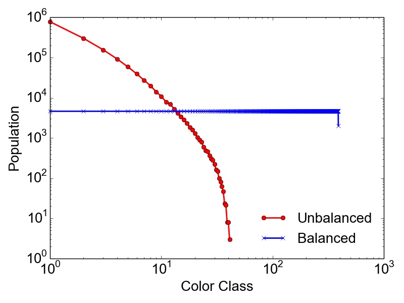
Therefore, it is common to evaluate the population of the color classes created by a graph coloring algorithm. In principle, there exist two types of solutions regarding the population of the color classes: (1) balanced and (2) unbalanced solutions. An equally balanced solution consists of \(n\) color classes with the same population. Obviously, it is in general impossible to always guarantee an equally balanced solution, except if \(k = n\). Thus, it is common to denote also a solution with an almost equally balanced coloring as a balanced solution. On the contrary, as most of the coloring algorithms aim at minimizing the used number of colors \(k\), their color class populations are most likely skewed, i.e., representing an unbalanced coloring solution. In order to compare the populations of the different color classes, the relative standard deviation (RSD) of the populations is used within this thesis:
\( \seteqsection {2} \) \( \seteqnumber {13} \)
\begin{equation} \text {RSD} = 100 \cdot \frac {s}{\bar {x}}. \label {eq:background:rsd} \end{equation}
Here, \(s\) denotes the standard deviation and \(\bar {x}\) the average population of the color classes. An example of a balanced and an unbalanced graph coloring solution obtained for a graph with 1,800,000 vertices and 19,000,000 edges, together with the corresponding RSD values, is depicted in Figure 2.4. The presented data prove that a balanced coloring usually requires more color classes than an unbalanced coloring. However, the balanced approach yields almost equitable color classes, where only the highest class(es) have smaller populations.
2.2 Meshes
This section introduces the necessary mathematical definitions in order to define what is commonly known as mesh. Furthermore, an introduction is given into numerous ways of describing the properties and qualities of meshes resulting from so-called mesh generation and mesh adaptation processes. The latter is subsequently subject to a more detailed analysis in the following section discussing common concepts and techniques to improve the quality of an already existing mesh.
In simplest terms, a mesh is a collection of non-dangling vertices, edges, and facets, discretely representing objects used, for example, in simulations or visualizations including physical objects, like semiconductor devices and structures [19], [21], [47]. To give a formal introduction into the topics of meshes and mesh adaptation, first some properties required for introducing a so-called simplex are given. A simplex is, informally, the simplest polytope in a given dimension [48].
-
Definition 2.2.1 (Affine Combination) [49] Let \(X=\{x_1, x_2, ..., x_k \}\) be a set of points in \(\mathbb {R}^d\). An affine combination of the points in \(X\) is a point \(p\) that can be written as \(p = \sum _{i=1}^{k} w_i x_i, \ \forall \ w_i: \sum _{i=1}^{k} w_i = 1\). A point \(p\) is called affinely independent of \(X\) if it is not an affine combination of points in \(X\). All points in \(X\) are affinely independent if no point in \(X\) is an affine combination of the others. The affine hull is the set of all affine combinations of points in \(X\).
-
Definition 2.2.2 (Convex Hull) [49] A point \(p\) that can be written as an affine combination with all \(w_i \geq 0 \ \forall \ i \in \{1,2,...,k\}\) is called a convex combination of the points in \(X\). The set of all convex combinations of points in \(X\) is the convex hull of \(X\), \(conv(X)\).
Figure 2.5 depicts exemplary finite point sets and their corresponding convex hulls.

-
Definition 2.2.3 (\(k\)-Simplex) [49] A \(k\)-simplex \(\sigma \) is the convex hull of \(k+1\) affinely independent points: \(\sigma =conv(S)\). The dimension of a \(k\)-simplex is \(dim(\sigma )=k\).
The above defined simplices are the convex hulls of finite point sets, where the simplest possible \(k\)-dimensional polyhedron is a \(k\)-simplex. Figure 2.6 shows a 3-simplex, i.e., a tetrahedron.
-
Definition 2.2.4 (Face) [49] A face of a \(k\)-simplex \(\sigma \) is a simplex that is the convex hull of a non-empty subset of \(X\). A proper face of \(\sigma \) is any face except \(\sigma \).
-
Definition 2.2.5 (Facet) [49] All \((k-1)\) faces of a \(k\)-simplex \(\sigma \) are the facets of \(\sigma \). Every \(k\)-simplex has \(k+1\) facets.

With the definition of a simplex and its faces and facets it is possible to describe sets of simplices, with the simplicial complex representing one of the most important sets.
-
Definition 2.2.6 (Simplicial Complex) [49] A simplicial complex \(K\) is a set of finitely simplices obeying two conditions:
-
1. \(K\) contains every face of every simplex in \(K\),
-
2. for any two simplices \(\sigma , \kappa \in K: \ \sigma \cap \kappa \leq \sigma ,\kappa \).
-
In the above definition the first condition ensures that if \(\sigma \) is part of a set of simplices also every face of \(\sigma \) is part of this set. The second condition states that the intersection of two simplices has to be empty or a face of both \(\sigma \) and \(\kappa \).
To discretize continuous physical objects it is possible to create a triangulation, which can be defined as follows.
-
Definition 2.2.7 (Triangulation) [50] A triangulation of a set \(V\) of points is a simplicial complex \(K\) whose vertex set is a subset or equal to \(V\), and the underlying space of \(K\) is the convex hull of \(V\).
This general definition of a triangulation allows for many different options to triangulate a given point set. Additionally, the definitions of a simplicial complex are used to define the triangulation. Thus, this definition is also valid for 3D discretizations using tetrahedra or hexahedra and these types of triangulation in three dimension are called tetrahedralizations and hexahedralizations, respectively. Note also that every point set can have a triangulation [49].
A prominent type of triangulation is the so-called Delaunay triangulation. Due to its beneficial properties and its dual representation (i.e., Voronoi diagram), it is widely used in science and engineering [49]. To define the Delaunay triangulation the definition of the circumsphere of a \(k\)-simplex is required first.
-
Definition 2.2.8 (Circumsphere) [50] For a given point set \(V \in \mathbb {R}^d\), and \(\sigma \) being a \(k\)-simplex with \(0 \leq k \leq d\), whose vertices are in \(V\), the circumsphere of \(\sigma \) is a sphere that passes through all vertices of \(\sigma \).
-
Definition 2.2.9 (Delaunay Property) [50] A \(k\)-simplex is Delaunay if there exists a circumsphere of \(\sigma \) such that no vertex of the point set \(V\) lies inside it.
With these definitions it is now possible to define the Delaunay triangulation for point sets in dimension \(d \geq 1\).
-
Definition 2.2.10 (Delaunay Triangulation) [50] Let \(S\) be a finite point set in \(\mathbb {R}^d\) and \(k\) be the dimension of its affine hull. A Delaunay triangulation of \(S\), \(Del(S)\), is a triangulation of \(S\) such that all \(k\)-simplices are Delaunay.
Figure 2.7 depicts an example of a Delaunay triangulation.

Although there are different definitions of a mesh and a triangulation used in the literature, here a mesh is considered to be a special type of a triangulation: For the latter the boundary information of the domain is lost [51]. For example, if the geometry to be triangulated consists of a hole, a triangulation will also fill this hole with elements. Thus, elements outside of the original geometry, e.g., covering a hole, have to be removed in a subsequent step. However, a mesh aims at preserving the explicit domain information while constructing a triangulation.
-
Definition 2.2.11 (Conforming Mesh) [51] Let \(\Omega \) be a closed domain in \(\mathbb {R}^d\), with \(d \in \{2,3\}\) and \(\sigma \) a mesh element, i.e., a simplex. Then \(M\) is a mesh of \(\Omega \) if
-
1. \(\Omega = \frac {\circ }{\underset {\sigma \in M}{\bigcup } \sigma }\).
-
2. The interior of every element \(\sigma \) in \(M\) is non-empty.
-
3. The intersection of the interior of two elements in \(M\) is the empty set \(\emptyset \), or a face.
-
The first condition guarantees that the boundary is preserved and the second condition that elements do not overlap. The last condition ensures that if two elements are not adjacent their intersection is empty, whereas the intersection of adjacent elements results in a common face, e.g., a vertex. Examples of both a conforming and a non-conforming mesh are depicted in Figure 2.8. Conforming meshes are particularly important for numerical simulations, e.g., FEMs or FVMs, in order to correctly compute PDE solutions for arbitrarily shaped simulation domains.


2.2.1 Mesh Quality
Assessing the quality of a generated or already existing mesh is a key step in order to guide a potentially subsequent mesh adaptation process, where the main goal is to increase the mesh quality and thus the solution accuracy and quality of FEM/FVM-based simulations. Therefore, it is first necessary to define the quality of a mesh. This can be achieved by using numerous different metrics for 2D and 3D meshes [52], [53], [54].
One of the most popular quality metrics for 2D triangular as well as 3D tetrahedral meshes is the minimum angle present in a mesh element. The minimum angle for triangles is measured between two edges and for tetrahedra between two triangular facets. Equilateral triangles and equilateral tetrahedra yield minimum angles of \(60^\circ \) and \(70.53^\circ \), respectively [54].
Another important quality metric is the edge ratio defined as
\( \seteqsection {2} \) \( \seteqnumber {14} \)
\begin{equation} R_{\text {edge}} = \frac {L_{\text {max}}}{L_{\text {min}}}, \label {eq:background:edge_ratio} \end{equation}
where \(L_\text {max}\) and \(L_\text {min}\) is the maximum and the minimum edge length of a triangular or tetrahedral mesh element, respectively. Optimal elements, i.e., equilateral elements, have an edge ratio of \(R_{\text {edge}}=1\) [54].
However, the distribution of any mesh quality metric does not guarantee the convergence of numerical solutions obtained by FEMs/FVMs, as a single low quality element can jeopardize the solution. For example, large angles yield large discretization errors, i.e., large differences between the computed and the true solution. Furthermore, small angles result in ill-conditioned matrices. Additionally, the size as well as the number of mesh elements affect both the accuracy of the solution and the computation costs required for the solution of the PDE [49].
2.2.2 Mesh Adaptation
The main goal of mesh adaptation is to improve the quality of the mesh elements and thus subsequently the mesh as a whole with respect to certain prescribed demands. This can be achieved by utilizing two fundamentally different types of adaptations: 1) \(h\)-adaptivity, and 2) \(r\)-adaptivity. The first approach conducts the adaptation process by adapting the mesh topology, e.g., by adding new elements to the mesh increasing its resolution. In turn, \(r\)-adaptivity preserves the topology of an existing mesh and aims to improve the element quality by applying, for example, different vertex smoothing algorithms which relocate vertices [55].
2.2.2.1 Refinement
Refinement describes methods of increasing the local or global mesh resolution by adding elements to an existing mesh thus belonging to the group of \(h\)-adaptivity methods. Although the refinement procedure itself is potentially computationally expensive, the increase in computational costs is usually outweighed by a more exact solution of the PDEs [55].
Element refinement denotes either the process of splitting existing edges and subsequently subdividing the corresponding elements or vertex insertion methods creating new vertices, for example, in the interior of the elements or on their facets. Edge splitting is in most cases guided by a threshold for the edge length. If the edge is longer than the prescribed threshold, it is split by inserting a vertex. The new vertex can be inserted on the midpoint of the edge, or depending on a specific metric somewhere else on the edge. After the edge split step the mesh contains dangling vertices which have to be properly connected in a subsequent element subdivision step. An example of a template-based refinement scheme was presented by Li et al. [56], where the elements are subdivided based on the number of split edges. Thus, in two dimensions three principal different subdivision schemes for a triangular element are possible (see Figure 2.9). Similar procedures are available for 3D tetrahedral meshes, where the refinement operation can split one of the edges or insert a vertex on a facet of a tetrahedron [56].


2.2.2.2 Swapping
A mesh can contain numerous low-quality elements. Hence, edge swapping (sometimes called flipping) techniques aim at replacing these low quality elements with higher quality elements, improving the overall mesh quality. With this procedure the number of elements in the mesh remains constant.
The swapping operation in 2D meshes is conducted by so-called edge flips, where two adjacent cells are replaced by two new cells. Hence, swapping belongs to the \(h\)-adaptivity methods. An example of an edge flip is shown in Figure 2.10, where an edge shared between two triangles is flipped resulting in two higher quality triangles (i.e., triangles with balanced, larger angles). Swapping plays a key role in 2D meshing, as the edge flipping operations can transform any mesh into a Delaunay mesh [49]. However, extending the edge flipping operations from two to three dimensions, where they are called bistellar flips, is not a trivial task. Considering tetrahedral meshes, it cannot be guaranteed that the resulting mesh is Delaunay [49]. Additionally, if the 3D mesh is comprised of other element types, e.g., hexahedra or cubes, flipping is even more intricate [57].


2.2.2.3 Coarsening
Coarsening or decimation operations are \(h\)-adaptivity methods used to decrease the local resolution in a mesh by removing mesh elements. Two common ways of coarsening are the edge collapse and the element collapse. In the first, an edge comprised of two vertices is removed by collapsing the vertices into a single vertex. Hence, the two adjacent elements of the former edge are removed. An example of an edge collapse is depicted in Figure 2.11. The resulting local patch depends on the direction of the edge collapse, i.e., it is an orientated operation. The choice of which vertex is replaced can have a severe impact on the quality of the resulting elements. Thus, several approaches have been developed trying to compute the optimal location of the final vertex after the edge collapse operation [56], [58]. In 2D meshes the element collapse operation reduces a triangular mesh element into a single vertex, leading to the deletion of a total of four elements: The collapsed element and all adjacent elements which shared an edge with the collapsed element.


2.2.2.4 Smoothing
Vertex smoothing is an \(r\)-adaptivity operation applied in many mesh adaptation workflows in order to improve the mesh quality. The main idea behind smoothing is to relocate vertices without inserting or removing any elements. Thus, the connected elements are altered, aiming for a higher mesh quality. Due to their restriction of preserving the existing mesh topology, smoothing algorithms are usually easy to implement with respect to the underlying mesh data structures. One of the most popular smoothing algorithms is the Laplacian smoothing (see Figure 2.12) proposed by Field [59], which is also applicable for non-simplex meshes [60]. However, the relocation has to be constrained to prevent elements from being inverted and to preserve the conformity of the mesh to a prescribed geometry. As vertex smoothing is a popular mesh adaptation technique, numerous more complex algorithms have been published in the past. These include smart Laplacian smoothing [61], smoothing based on the optimal Delaunay triangulation [62], smoothing utilizing local quality metric optimizations [63], and smoothing guided by the solution of a constrained optimization problem [64].


2.3 Parallel Computers
This section covers a basic introduction into the architectures of modern processors and computer systems, which are critical for the developed high-performance computing approaches. After presenting the basic concepts of a computer architecture the principles of multi-core and multi-threaded processors are discussed. Finally, different parallelization principles and techniques are presented.
2.3.1 Basic Computer Architecture
The basic principle of computer systems used today was introduced by Alan Turing in the 1930s and brought to real life in the late 1940s by Ecker and Mauchly [65]. This so-called stored-program digital computer, depicted in Figure 2.13, splits the core functionality into three different main parts: 1) Input/Output functionality, 2) Memory, and 3) central processing unit (CPU). The latter is often simply referred to as processor or core and these terms are used interchangeably. Linking several CPUs (processors/cores) results in a so-called multi-core processor (see Section 2.3.1.1) [25]. One major advantage of this design is that all instructions are stored as data in the memory. The commands are then read and processed by the different building blocks of the CPU, i.e., control and arithmetic logic unit [25].

Figure 2.13: Main building blocks of the stored-program digital computer. The instructions residing in the memory are read by and executed on the control and arithmetic logic unit. The CPU also takes care of all input and output mechanisms (Adapted from [25]).
However, this simple design has some principle drawbacks. First, to utilize such a computer system efficiently both instructions and data have to be read by the CPU continuously. Hence, the limiting factor is the speed of the memory. This performance bottleneck is known as von Neumann bottleneck [66].
To alleviate this limitation, several methods for performance boosting have been invented. For example, the use of caches, which are fast but small on-chip memories residing between the CPU and the main memory. The cache stores previously or likely to be used data (prefetching) in order to provide those faster to the processor if necessary [67]. It is also possible to include more than one cache in an architecture, for example separate caches for data and instructions [25]. Figure 2.14 depicts another design using two levels of caches, where the level-1 cache is split into instruction and data cache. Additionally, it shows a major performance limiting factor, the DRAM gap, denoting the major bandwidth differences between main memory and caches [25].
Another option of improving the performance is pipelining. Pipelining is a concept, based on the subdivision of complex operations, e.g., floating point addition, into several easier to handle instructions that can be executed by the different units on the CPU in parallel. Thus, the total amount of instructions per time unit is increased [68].
The second major limiting factor of the stored-program computer design is that this architecture is only capable of processing a single instruction on a single operand (Single Instruction Single Data (SISD)). With the introduction of the first vector supercomputers, the idea of Single Instruction Multiple Data (SIMD) was born. SIMD executes the same instruction on more than a single operand, commonly on an array of integer or floating point operands [25].

Figure 2.14: A data-centric view of a cache-based computer design, using a level-1 (L1) and a level-2 (L2) cache. The L1 cache is split into data (D) and instruction (I) cache. The arrows indicate the data flow between the different units, with the DRAM gap describing the speed differences between main memory and caches. (Adapted from [25].)
2.3.1.1 Multi-Core Processor
In the last century, scientists and engineers could rely on the fact that the transistor count on a single computer chip is doubled almost every 24 months (known as Moore’s Law) [69], which translated to increased performance with every new CPU generation. In addition to the increase in transistor density also the clock frequency has increased steadily. However, a higher clock frequency yields an increase in power dissipation which is why both basically saturated around 2005 [70], [71].
Therefore, a new design has been introduced, featuring more than one processor or core on the same die; as transistor feature scales continue to shrink processor vendors are able to continue introducing more transistors with every new generation and use these to provide more processing cores. There exist different designs of placing multiple cores on a chip. Several examples of different multi-core designs are depicted in Figures 2.15 and 2.16. It is possible that every processor has its own dedicated caches (see Figure 2.15a), or share different higher cache levels (see Figure 2.15b and Figure 2.16).


Figure 2.15: Different examples of multi-core designs. The left shows a dual-core processor chip with dedicated cache levels for each processor. On the right, a quad-core processor is shown. It consists of a single L1 and a shared L2 chip for each processor. (Adapted from [25].)

Figure 2.16: Example of a hexa-core design consisting of a shared L3 cache, a dual-core shared L2 cache and a dedicated L1 cache for each processor. (Adapted from [25].)
The overall performance of any multi-core system can be calculated as [25]
\( \seteqsection {2} \) \( \seteqnumber {15} \)
\begin{equation} p_m = (1+\varepsilon _p)\cdot p \cdot m, \end{equation}
where \(\varepsilon _p=\frac {\Delta p}{p}\) denotes a relative change in performance stemming from a change in clock frequency, with \(p\) being the performance of a single processor, and \(m\) being the number of processors present in the multi-core system.
In order to build a useful multi-core system from slower processors, the relative change in performance \(\varepsilon _p\) should obey
\( \seteqsection {2} \) \( \seteqnumber {16} \)
\begin{equation} \varepsilon _p > \frac {1}{m}-1, \end{equation}
meaning that at least the single-core performance is matched. A multi-core system comprised of \(m\) processors does not achieve \(m\) times the performance of a single-core unit, mostly because of issues resulting from non-optimal cache use, limited memory bandwidth in memory-bound problems, or non-optimal load-balancing [25]. However, to get the most performance out of multi-core systems it is absolutely necessary to efficiently tailor any program using parallel programming techniques to the underlying hardware (see Section 2.3.2).
2.3.1.2 Multi-Threaded Processor
In modern computer systems the different execution speeds of the various components, e.g., main memory execution speed is way cache speed, potentially leave major parts, like caches or registers, idle during program execution. To alleviate this problem concepts like pipelining have been introduced and applied to all modern CPU architectures. However, longer pipelines, raising clock frequency, and increasing problem complexity eventually yield a higher increase in power dissipation. This effect is only partially avoided by creating multi-core systems [25].
Therefore, the main goal in order to boost the computing performance is to decrease the idling times of the different CPU units. Simultaneous multi-threading (SMT), sometimes called (multi-)threading, is based
on the fact that a processor’s architectural units, such as data registers, are available multiple times.
Thus, these units can be viewed as several logical cores on a single physical core (depending on the degree of replication). On the contrary, the execution units, like arithmetic units or caches, are not replicated. Based on
the available multiple architectural states it is possible to execute several instruction streams, or threads, in parallel. Therefore, if one thread is idling, another thread can use the available resources, like data registers, leading to an
increase in overall computational efficiency. Unfortunately, a serial program does not necessarily benefit from this multi-threaded approach but is most likely experiencing a decrease in performance, especially if multiple different
serial programs are executed in parallel. One reason for this performance decrease can be an increasing number of cache misses, e.g., necessary data not being present in the cache or being invalid, leading to more data read
operations in the main memory, especially if two threads share the same cache. Additionally, if two threads are idle and wait for the same resource to be freed the overall performance will suffer from this synchronization
penalty [25].
2.3.2 Parallel Programming
In Section 2.3.1 the SIMD concept has been introduced, which is nowadays one of the two dominating approaches regarding parallel architectures. SIMD is applied in modern graphics processing units (GPUs) [72] or vector processors [73]. Another parallelization concept is Multiple Instruction Multiple Data (MIMD), utilizing different instruction streams working on different data sets. These concurrent instruction sets run on different processors in parallel. Two modern parallel computer architectures, i.e., shared-memory and distributed-memory systems, are two examples following the MIMD concept [25]. These two parallel architectures can be combined forming so-called hybrid systems. Additionally, as will be discussed, so-called accelerators (or coprocessors) are available, providing specialized parallel computing platforms with high core counts and memory bandwidths.
2.3.2.1 Shared-Memory Systems
Following a basic definition, a shared-memory parallel computer consists of multiple processors working on a shared physical address space [25]. Depending on the detailed architecture, the shared-memory systems can be further divided into two main categories:
-
1. Uniform Memory Access (UMA) systems, and
-
2. (cache-coherent) Non-Uniform Memory Access ((cc)NUMA) systems.
The main principle behind UMA systems is to guarantee equal latency and bandwidth for all processors and all memory locations. A simple design of a UMA system consisting of four cores is depicted in Figure 2.17. Here, the four processors use the same path to the memory. The limited memory bandwidth is a major drawback of the UMA design, making it hard to build scalable UMA systems consisting of 16 or more CPUs [25].

However, in modern computer systems more than a single socket are common, yielding a higher complexity and higher demands on the connecting memory. Thus, a different design giving up the UMA approach, i.e., the (cc)NUMA design, alleviates these drawbacks. Here, each processor has its own memory and is grouped into a locality domain. The locality domains are coherently linked to provide a unified shared-memory access. An example of such a design is depicted in Figure 2.18. (cc)NUMA architectures are very scalable and are thus used for high-performance computing clusters and supercomputers [25].

Figure 2.18: An example of four locality domains comprising a (cc)NUMA system, each containing a dedicated processor and its memory. The different domains are linked using an interconnect. Memory access times differ depending on the locality domain where the requested data or instructions are stored, i.e., if they reside in a different domain [74].
However, as a drawback, (cc)NUMA architectures require software developers to consider potential non-local memory accesses: Accessing data via cache-coherent links (necessary if data is not in a thread’s locality domain) triggers performance penalties. This so-called locality problem can result in a performance penalty even for serial programs [74]. A second issue potentially limiting performance is contention and appears if two processors in different locality domains try to access memory in the same locality domain and thus compete for the available memory bandwidth. Resolving these two issues is crucial to obtain optimal performance for an application and has to be ensured by keeping the data access of each processor inside its locality domain as much as possible.
For both of the above systems (i.e., UMA and (cc)NUMA) it is absolutely necessary to keep all copies of the same cache data, which can be present in multiple caches of different CPUs, consistent. Hence, so-called cache coherence protocols ensure the consistency between cached data and data residing in the memory, e.g., the outdated but conceptually representative MESI protocol [75].
From the software perspective, developing efficient parallel source code becomes more and more challenging due to the increasingly complex (cc)NUMA architectures. Therefore, shared-memory tailored parallelization libraries are
available to aid the software developer. These include software libraries like OpenMP [76], [77], Intel Cilk Plus [78], pthreads [79], and TBB [80]. To obtain a reasonable scaling on shared-memory systems the data access
patterns and the operations to be conducted in parallel have to be rigorously optimized. Although the main idea of allowing threads to access the same memory address space is convenient, performance penalties from NUMA effects
can easily jeopardize a potential performance gain. Another common problem occurring on shared-memory systems is, if two threads utilize different operations with data from the same memory address. It can happen that the
results of these computations differ depending on the specific order of the actual instructions (race condition). Further, if, for example, two threads write their different results to the same memory location, it cannot be guaranteed
which result will eventually be stored in the memory. This is called a data race situation [25]. To avoid this problem, the
code sections possibly leading to data races, can be marked as critical sections. Inside a critical section only a single thread is allowed to execute this specific fraction of code. All other threads have to wait for the executing thread
to actually exit the critical section. However, if two threads inside different critical sections wait for the other thread to exit its critical section before continuing, actually no thread is able to continue.
This so-called deadlock yields a stop in program execution. Nevertheless, over-using critical sections creates potential performance bottlenecks or even leads to situations where the program execution has to be
aborted [81].
2.3.2.2 Distributed-Memory Systems
Another important parallel computing architecture is distributed-memory. The main idea behind this architecture is the use of independent processors connected via a network, each having exclusive access to its own memory, as shown in Figure 2.19. However, remote access to another processor’s memory requires explicit network communication (contrary to shared-memory approaches, where memory access is implicitly possible).

Strictly speaking, the design of individual processors building a distributed-memory system (Figure 2.19) is nowadays obsolete and reflects more or a less only a programming model. This is due to the fact that in every modern high-performance computing cluster the principle building blocks consist of shared-memory nodes, comprised of multiple multi-core CPUs. However, a distributed-memory programming model can also theoretically be utilized on such a single shared-memory node [25]. The most common programming model for distributed-memory programming is the so-called Message Passing Interface (MPI) [82], [83]. However, other programming models are available, e.g., High-Performance Fortran [84], [85], and partitioned global address space models [86] like Unified Parallel C [87], [88].
In contrast to shared-memory programming models, distributed-memory models build on processes instead of threads [25]. Due to the fact that processes have exclusive access to their corresponding memory address spaces, the data and information exchange via the network interface is performed in MPI using messages [82]. Hence, the specific hardware layout as well as the processing speed and capabilities of the network interfaces have a direct influence on the overall parallel performance in a distributed-memory system.
2.3.2.3 Hybrid Systems
As mentioned above no modern high-performance computing cluster is neither shared-memory nor distributed-memory only. Commonly, shared-memory compute nodes with multiple multi-core CPUs make up the single building blocks in a bigger distributed-memory environment interconnected via a network.
From a software point of view, in most cases these hybrid systems are utilized using distributed-memory programming models, in particular MPI [25]. However, some computational problems might benefit from an efficient utilization of the shared-memory on the individual nodes of a distributed-memory system, i.e., combining distributed- and shared-memory approaches. For example, MPI can be used to take care of all inter-node communication and the available on-node parallelism can be exploited using OpenMP. Examples of such approaches can be found in the fields of mesh smoothing [89], geomechanics [90], and fluid mechanics [91].
2.3.2.4 Accelerators
Aside from multi-core CPUs, other high-performance computing platforms are accelerators, particularly suitable for SIMD operations. These include GPUs as well as coprocessors. For example, the Summit supercomputer of IBM [92] uses Nvidia Tesla V100 GPUs, which are dominantly programmed using CUDA [93], whereas the Tianhe-2 is equipped with Intel Xeon Phi 31S1P coprocessors [94]. One of the major advantages of accelerators is their excellent energy consumption to performance ratio compared to standard shared-memory compute nodes at the price of being tailored to specific computational problems and requiring additional data transfers to the accelerators’ own memories. Due to their significant acceleration potential, accelerators are used for example in the fields of life sciences [95] and deep learning [96].
2.3.2.5 Basics of Parallelization
There are different types of parallelism available besides the already mentioned fine-grained SIMD methods found for example on GPUs. One approach is called data parallelism and is the most prominent type of parallelization in scientific computing [97]. An example of data parallelism is the physical simulation of mechanical systems, where the simulation domain is represented with a mesh. By using a process called domain decomposition, which splits the initial mesh into smaller partitions, it is possible to assign each partition to individual cores, thereby realizing parallelization: The individual partitions are processed in parallel. This approach can be utilized on both shared-memory and distributed-memory systems. Regardless, the parallel efficiency strongly depends on the exact domain decomposition: The goal is to provide partitions containing the same amount of work (load balancing), however, this is not always possible. Additionally, it is important to reduce the necessary communications between the different partitions, which depends on the locality of the data itself. Thus, it becomes vital to create data access and transfer patterns benefiting from data locality to maximize parallel efficiency [25].
To effectively measure the parallel performance of a program, the serial (\(s\)) and parallel (\(p\)) parts need to be put into relation:
\( \seteqsection {2} \) \( \seteqnumber {17} \)
\begin{equation} s + p = 1. \label {eq:work} \end{equation}
Considering the optimal case, using \(n\) processors would reduce the runtime \(T\) of solving a certain task to \(T/n\). However, there are limitations to the achievable parallelization efficiency. These include intrinsic limitations of the algorithm, such as data dependencies, shared resources, e.g., shared memory, or communication between the different processors. If the total amount of work stays constant and \(n\) processors are used, the overall serial time of Equation 2.17 reduces to
\( \seteqsection {2} \) \( \seteqnumber {18} \)
\begin{equation} T_p=s+\frac {p}{n}. \end{equation}
This approach of measuring the parallel performance is known as strong scaling. It aims at minimizing the overall runtime for a given problem size. However, if the overall runtime is not of importance, because memory performance is the dominating limitation, it is necessary to introduce a scaling factor \(\alpha \). \(\alpha \) keeps the amount of work performed by each core identical for any number \(n\) of computational cores. This approach is called weak scaling:
\( \seteqsection {2} \) \( \seteqnumber {19} \)
\begin{equation} T_s^{\alpha } = s + pn^\alpha . \end{equation}
It follows that the resulting parallel runtime for \(n\) workers is
\( \seteqsection {2} \) \( \seteqnumber {20} \)
\begin{equation} T_p^\alpha = s + pn^{\alpha -1}. \end{equation}
After introducing two of the most common scalability measures, it is clear that regardless how well a given task is parallelized, there will always be a serial fraction, limiting the parallel performance gain. Let now the total amount of work introduced in Equation 2.17 be expressed as \(T_s\). Then the parallel performance for a fixed problem size can be written as
\( \seteqsection {2} \) \( \seteqnumber {21} \)
\begin{equation} P_s = \frac {s+p}{T_s} = 1. \end{equation}
Subsequently, the parallel performance evaluates to
\( \seteqsection {2} \) \( \seteqnumber {22} \)
\begin{equation} P_p = \frac {s+p}{T_p} = \frac {1}{s+\frac {1-s}{n}}. \end{equation}
Looking at the ratio of the parallel to the serial performance, which is denoted as speedup (S), yields
\( \seteqsection {2} \) \( \seteqnumber {23} \)
\begin{equation} S = \frac {P_p}{P_s} = \frac {1}{s+\frac {1-s}{n}}. \label {eq:amdahl_law} \end{equation}
Equation 2.23 is known as Amdahl’s law [98]. This simple equation states that the optimal speedup of any parallelization task is limited by the amount of serial work as for \(n \rightarrow \infty \) Equation 2.23 evaluates to \(\frac {1}{s}\). Note that this fact is only valid for strong scaling cases, where the problem size remains constant. For weak scaling problems the obtainable speedup is
\( \seteqsection {2} \) \( \seteqnumber {24} \)
\begin{equation} S_\text {weak}=1+\frac {p}{s}n^\alpha , \ \ \ 0 < \alpha < 1. \end{equation}
Ideal weak scaling would result in \(\alpha =1\), yielding
\( \seteqsection {2} \) \( \seteqnumber {25} \)
\begin{equation} S_\text {weak}=s+(1-s)n. \label {eq:gustafson_law} \end{equation}
This equation is known as Gustafson’s law [99]. Note that due to the linearity of \(n^\alpha \) it is theoretically possible for weak scaling problems to get unlimited performance.
2.4 Benchmarking Platforms
In order to conduct a detailed investigation of the evaluated approaches and algorithms presented in this work, particularly focusing on their computational performance, two different benchmarking platforms (BPs) are used. The first one is a shared-memory node of the Vienna Scientific Cluster 3 (VSC-3). The second one is an accelerator, i.e., an Intel Xeon Phi coprocessor. The specific properties of the two test beds are listed below.
- BP1
-
A single node of VSC-3 is comprised of two Intel Xeon E5-2650v2 Ivy Bridge CPUs with eight cores at 2.6GHz and a total of 64GB main memory [100].
- BP2
-
A special node of VSC-3 containing an Intel Xeon Phi 7210 Knights Landing coprocessor, having 64 cores at 1.3GHz and in total 213GB main memory [100].
Table 2.1 contains a detailed overview of the hardware equipment of each BP.
| BP1 | BP2 | |
| Frequency [GHz] | 2.60 | 1.30 |
| Sockets | 2 | 1 |
| Cores per CPU | 8 | 64 |
| Main Memory (GB) | 64 | 213 |
| L1 Cache Size | 8 \(\times \) 32kB Instruction | 64 \(\times \) 32kB Instruction |
| 8 \(\times \) 32kB Data | 64 \(\times \) 32kB Data | |
| L2 Cache Size | 256kB | 32MB |
| L3 Cache (shared) | 20MB | — |
| Max. Bandwidth [GB/s] | 51.2 | 102 |
Table 2.1: Hardware overview of the two different benchmarking platforms.