5 Material Interface-Aware Surface Mesh Partitioning for Process TCAD
Numerical simulations typically impose two contradictory demands on the discretizations: (1) The meshes have to be accurate enough to correctly capture the physical properties and behavior of the investigated quantity distributions, and (2), they have to be coarse enough in order to reduce the simulation runtime as much as possible. Furthermore, Process TCAD simulations are categorized in two different major types, i.e., reactor-scale and feature-scale simulations. Reactor-scale simulations focus on simulating the entire reactor chamber, whereas the feature-scale approach utilizes a small fraction of the wafer surface region as simulation domain. The latter method is favored if a detailed description of the topographical behavior and an accurate prediction of the surface evolution is of interest [197], [198].
One type of feature-scale simulation in Process TCAD is the simulation of etching processes. Here, the vast number of possible process parameters and available materials renders conventional experimental evaluation unreasonable considering costs and time [2], since a slight change of a parameter in an experimental evaluation setup can have a critical impact on the properties of the resulting device [199]. Furthermore, as the evolution of the device designs yields more and more 3D designs, e.g., 3D FinFET [200] or 3D NAND flash memory [201], one approach of reducing the problem from three to two dimensions, as one of the simplest but most effective techniques to reduce the computational complexity of the simulations, becomes infeasible. Therefore, especially in TCAD, the development of more effective and faster algorithms became an important research focus to solve the increasingly complex 3D problems and thus contributes to sustaining the high pace of ultra scaled, integrated circuit developments [2].
Feature-scale etching simulations utilize, for example, a rectangular region of the wafer surface representing all geometrical features forming a device. Reflective or periodic boundary conditions model the physical behavior on the lateral boundaries of the domain. To model the gas particle species utilized in an etching process, a source plane is modeled at the top of the simulation domain. This source plane contains information about the angular and energetic distributions of the gases and effectively models the reactor chamber. The topographical changes in each timestep of an etching simulation are calculated using pre-defined physical models for the local etch rates or surface velocities. To calculate these surface velocities, the particle transport to the surface has to be computed, e.g., using ray tracing [198], resulting in a surface rate distribution for each considered particle species. For neutral particles and for ions these surface rates are included in the surface velocities as flux rate and sputter rate, respectively. Since the pressure inside a reactor chamber is quite low, ballistic transport models for the particles are used neglecting particle-particle interactions [198]. To model the particle transport different methods are used in etching simulations. A so-called bottom-up approach uses a discretized surface and computes the incoming flux for each surface mesh element using numerical integration over the angles under which the source plane is visible. The top-down approach is also based on a discretization of the surface but the particles are generated randomly on the source plane guided by the angular and energetic distributions of the particle sources. In an etching simulation the particle transport has to be computed in every single timestep and is the most time consuming part in each timestep. After computing the surface velocities, the advection of the surfaces is typically conducted using level-set based methods, as they can handle topological changes [198].
Feature-scale etching simulations using a level-set method for the surface advection can be split into different computational tasks: (a) preparation of a proper surface representation for the subsequent surface flux rate computation, (b) the calculation of the surface flux rate distributions on the surface, (c) the evaluation of the surface velocity models using the surface flux rate distributions, and (d) the advection of the surface according to the computed surface velocity field. The calculation of the flux rates is the most time-consuming part of an etching simulation [202], [203]. In turn, the mathematical models for the etch rates utilized in an etching simulation depend on the flux rate of the involved etchants, where the major computational bottleneck is induced by the flux rate calculations itself.
The aim of this chapter is to give an overview of existing methods and techniques aiming at improving the computational performance of flux calculation approaches in Section 5.1. This is followed by the description of an exemplary semiconductor fabrication process, i.e., the Dual-Damascene process, in Section 5.2 and the utilized multi-material representation in Section 5.3, which is capable of representing and advecting sub-grid resolution material layers. Since the Dual-Damascene process is a multi-material process and includes also etching processes it serves as a suitable example to prove the feasibility of the subsequently devised iterative partitioning method for multi-material surface meshes in Section 5.4 [17]. The evaluation of the newly introduced partitioning technique, with respect to performance and accuracy, is presented in Section 5.5 [17]. Eventually, Section 5.6 concludes the present chapter.
5.1 Related Work
Flux calculation methods based on ballistic particle transport require ray-surface intersection tests [198]. Level-set based surface advection approaches favor an implicit surface representation, because it inherently fits the level-set representation and support topological changes [204], [205], [206]. For example, Pagazani et al. investigated the so-called Bosch process, a highly anisotropic dry etching process used to create structures with high aspect ratios, for micro-electromechanical systems applications [207]. The authors use the commercial Victory Process simulator provided by Silvaco [208], which uses an implicit surface representation. Additionally, it is possible to use different temporary surface representations, e.g., an explicit representation, during ray casting. Another investigation of the Bosch process presented by Ertl and Selberherr is based on the open source ViennaTS simulator [209], [210]. Herein the process is simulated in three dimensions while the conducted flux calculation is based on a Monte Carlo method. Sets of overlapping disks are used to derive an approximative representation of the investigated surfaces. A different method for accelerating Monte Carlo based flux calculations was introduced by Heitzinger et al [211]. The main idea is to simplify the explicit surface representation, i.e., the mesh, in order to decrease the number of surface elements. Hence, the computational performance of the flux calculation step is increased as the number of elements to evaluate is decreased. However, mesh coarsening is computationally expensive and can pose an unwanted performance bottleneck as well as alter the geometry. Yu et al. presented a 3D topography simulation of a deep reactive ion etching process [212]. The authors use sets of spheres representing an approximation of the surface during the Monte Carlo ray tracing process, similar to the disks used by Ertl et al. [210].
In order to increase the computational performance of the conducted ray casting operations, one approach is to utilize hierarchical acceleration structures, such as the bounding volume hierarchy method [213], [214]. Yu et al. proposed a similar technique applying a bi-level spatial subdivision scheme in order to reduce the search space for an explicit surface representation [215]. This method relies on a proper subdivision tree and an optimal choice of the underlying parameters, which need to be determined beforehand. Such an optimal parameter set thus accelerates the conducted Monte Carlo based ray tracing as the performance of the ray-surface intersections is improved. A different acceleration technique was proposed by Naeimi and Kowsary for their heat transfer model [216]. The authors suggest to merge empty voxels, which are used to explicitly model their investigated geometry, inside their static simulation domain, reducing the overall number of voxels. Thus, when a ray traverses through the simulation domain, the empty areas are traversed faster, since the merged empty voxels are larger than those representing the actual surface. This algorithm delivers considerable speedup for the conducted ray tracing, but the merging process for the empty voxels can severely affect the overall performance of simulations, as it has to be conducted in every single timestep.
An approach for reducing the computational effort in radiosity-based flux calculations was introduced by Aguerre and Fernández [217]. Using explicit meshes, the acceleration method utilizes a hierarchical strategy combined with a sorting scheme to obtain accelerated flux calculations. Bailey proved that using an adaptive sampling method of the geometrical elements present in a simulation domain improves the computational performance of ray tracing operations [203]. Manstetten et al. showed that using temporary explicit meshes extracted from an implicit level-set based representation yield increased performance for single-precision ray-casting [218]. Furthermore, the authors showed that the introduced overhead of the conversion from the implicit to the explicit representation in each timestep is compensated by using optimized computer graphics libraries.
In a recent publication Manstetten et al. (together with the author of this thesis) introduced an acceleration approach increasing the computational performance for the flux calculation by evaluating the surface speeds only on a sparse set of mesh elements explicitly representing a surface [202]. To create this sparse set an iterative partitioning scheme for the surface is applied, without adapting the surface mesh elements themselves. The presented method is evaluated using a 3D single-material etching simulation of a cylindrical hole, a common structure in Process TCAD. An increase in performance for the flux calculation by a factor of 2-8 is reported depending on the level-set resolution, compared to the conventional evaluation using the whole set of surface mesh elements, with the advantage of preserving the geometrical features of the investigated surface. In what follows, the fundamental method is extended for handling multiple materials [17].
5.2 Dual-Damascene Process
A standard process used in the semiconductor industry, is the Dual-Damascene process which was introduced in the 1990s. The main goal of this process is the reduction of the required processing steps in a fabrication pipeline, yielding faster and cheaper production cycles [219]. As etching is an integral part of this process, it acts as a suitable example for evaluating Process TCAD simulations with a particular focus on etching.
The Dual-Damascene process requires only a single metal deposition step simultaneously filling both, vias and trenches using copper as a typical filling material [220]. A further advantage of this process is that the overall number of chemical-mechanical planarization as well as the number of necessary deposition steps for the inserted dielectric are reduced. Thus, the fabrication time is improved in addition to the reduced possibilities of failures due to the decreased number of processing steps.
Generally, the Dual-Damascene process is divided into three different processing sequences: (1) trench-first, (2) via-first, and (3) self-aligned (or buried-via). In the trench-first sequence the etching of the trenches is done before the vias are etched. In the via-first approach the etching of vias and trenches is conducted vice versa. Both methods have in common, that they apply a metal deposition step after each etching step, filling both via and trenches with copper. Contrary to those two methods, the self-aligned Dual-Damascene processing sequence etches the vias as well as the trenches at the same time [219], [221]. The self-aligned process is the example application to evaluate the multi-material interface-aware iterative partitioning method detailed in Section 5.4.
The single steps of an exemplary self-aligned Dual-Damascene process are depicted in Figure 5.1 with the different materials denoted with different colors (Figure 5.1a). The initial wafer surface is depicted in Figure 5.1b. The second processing step is the deposition of the diffusion barrier, followed by a dielectric and an etch stop layer (Figure 5.1c). The processing sequence is continued by the deposition of a hard mask and subsequently an additional etch stop layer is patterned (Figures 5.1d-5.1e). After removing the hard mask, another dielectric layer is deposited and again a hard mask is patterned (Figures 5.1f-5.1g). Afterwards, the key processing step of the self-aligned Dual-Damascene process is conducted: The combined etching of the trenches and vias as depicted in Figure 5.1h. This is followed by the removal of the remaining diffusion barrier layer (Figure 5.1i) and the deposition of the metal seed layer (Figure 5.1j). Finally, the processing sequence is finished by a copper deposition (Figure 5.1k) and a chemical-mechanical planarization step (Figure 5.1l).
Especially after switching the interconnect material from aluminum to copper in the beginning of the 21\(^{\text {st}}\) century as one of the many steps to overcome the challenges in the sub-micron regime [219], new challenges arise today on the way to further miniaturize semiconductor devices to a few nanometers and beyond. Among the many challenges is to reduce the interconnect capacitance. This is achieved by applying new dielectric materials, e.g., porous SiCOH [222]. Thoroughly designed and conducted computer simulations help to asses the different etching behaviors of numerous new materials to determine processing patterns and optimization strategies, before proceeding with cost and time-consuming conventional experimental investigations. Thus, especially the etching steps of a dielectric layer, as shown in Figures 5.1g5.1h, prove to be a practically highly relevant test case for the evaluation of new or adapted computational methods and are thus used in this work.
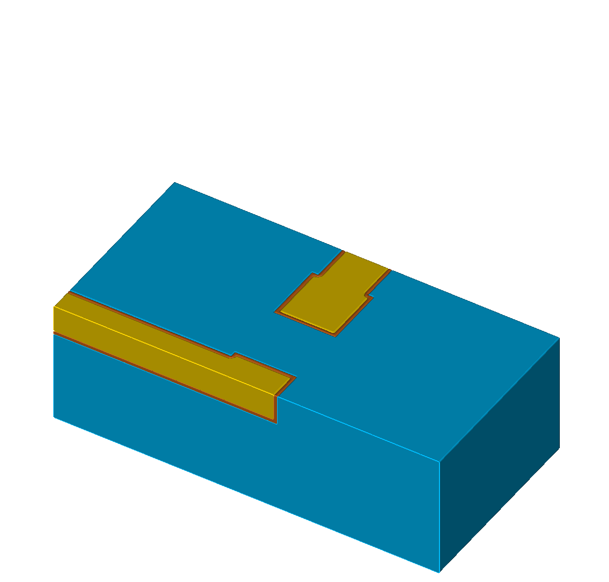
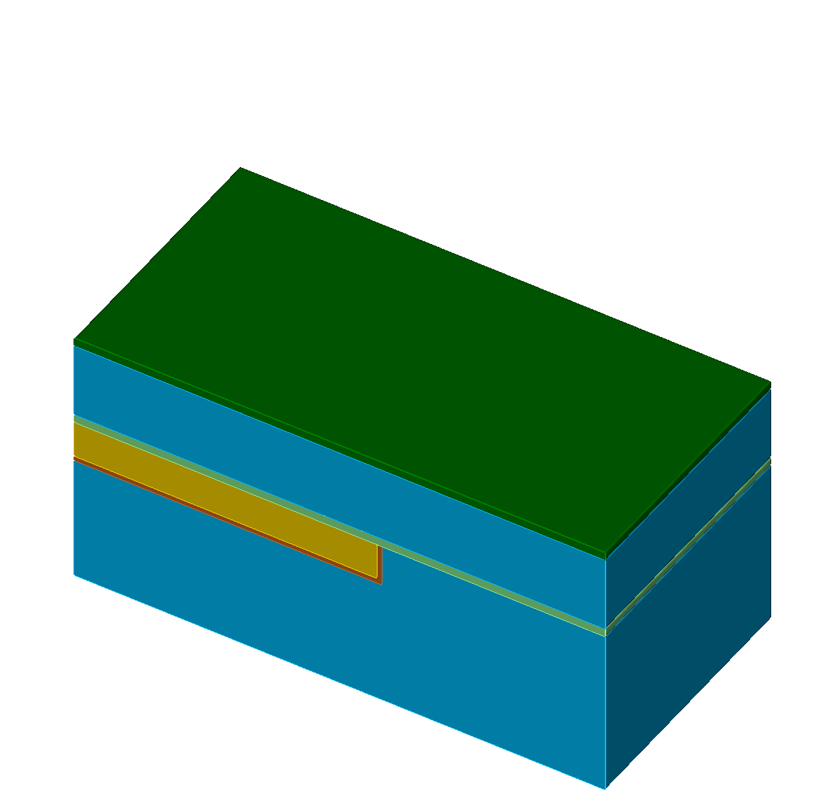
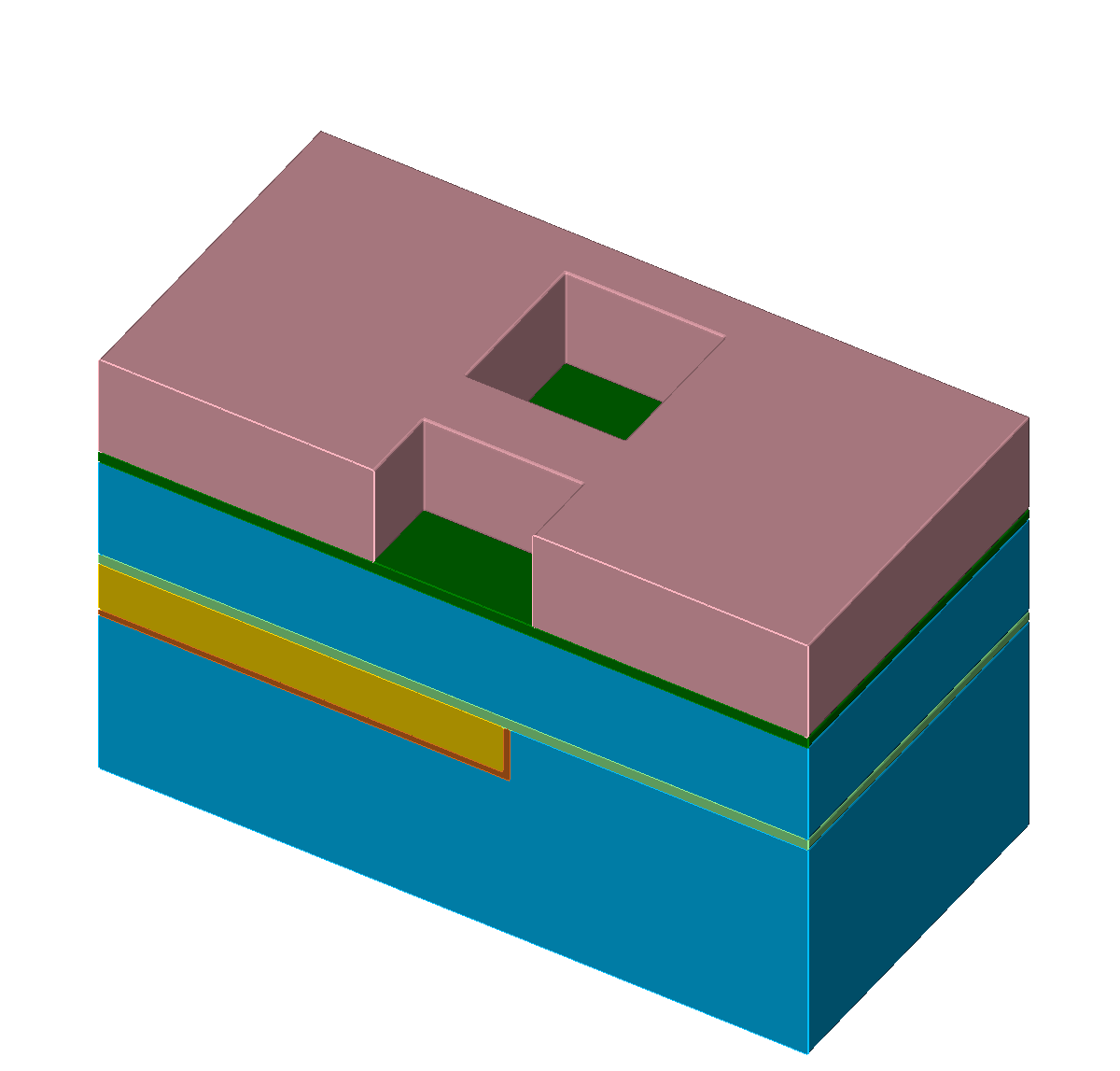
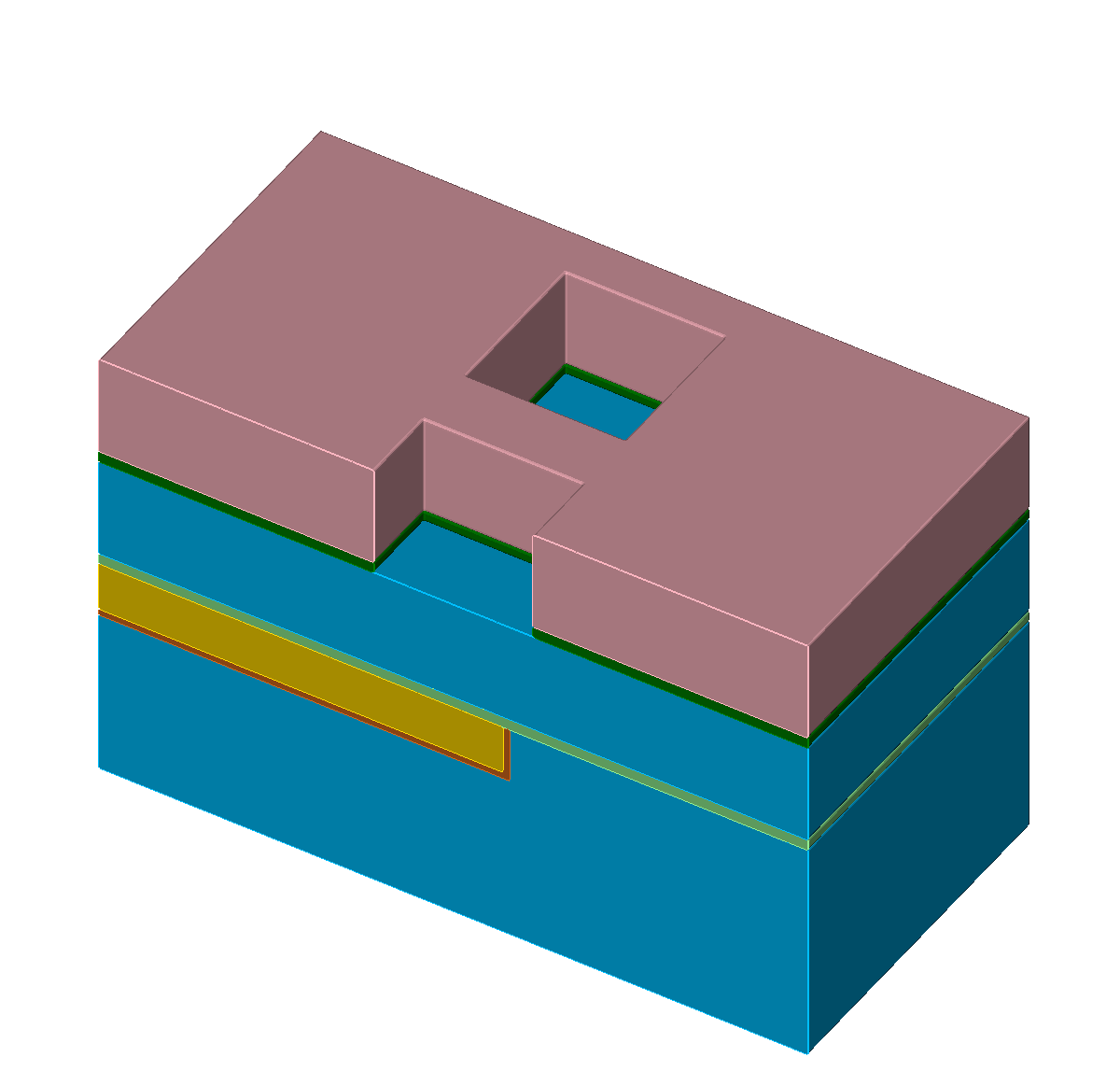
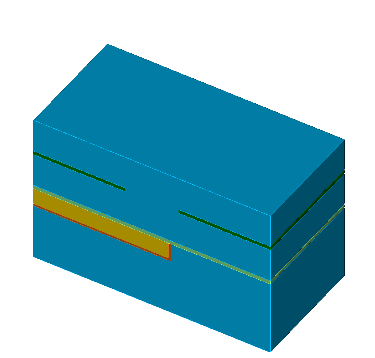
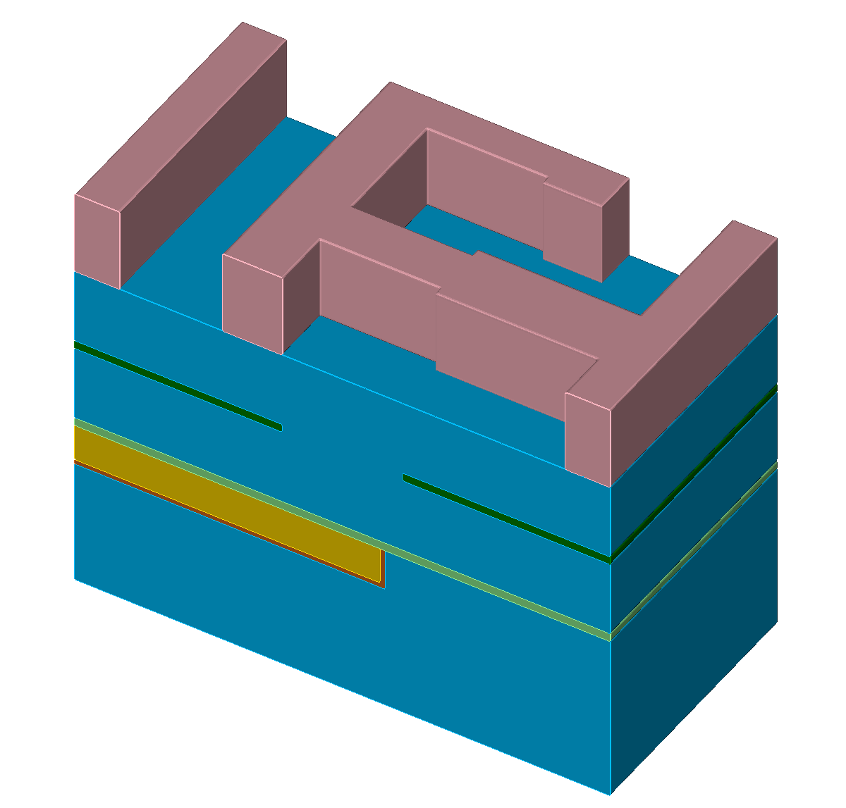
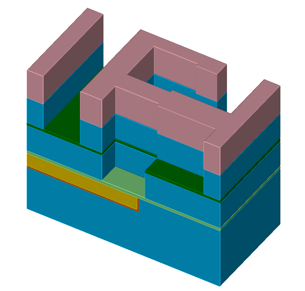
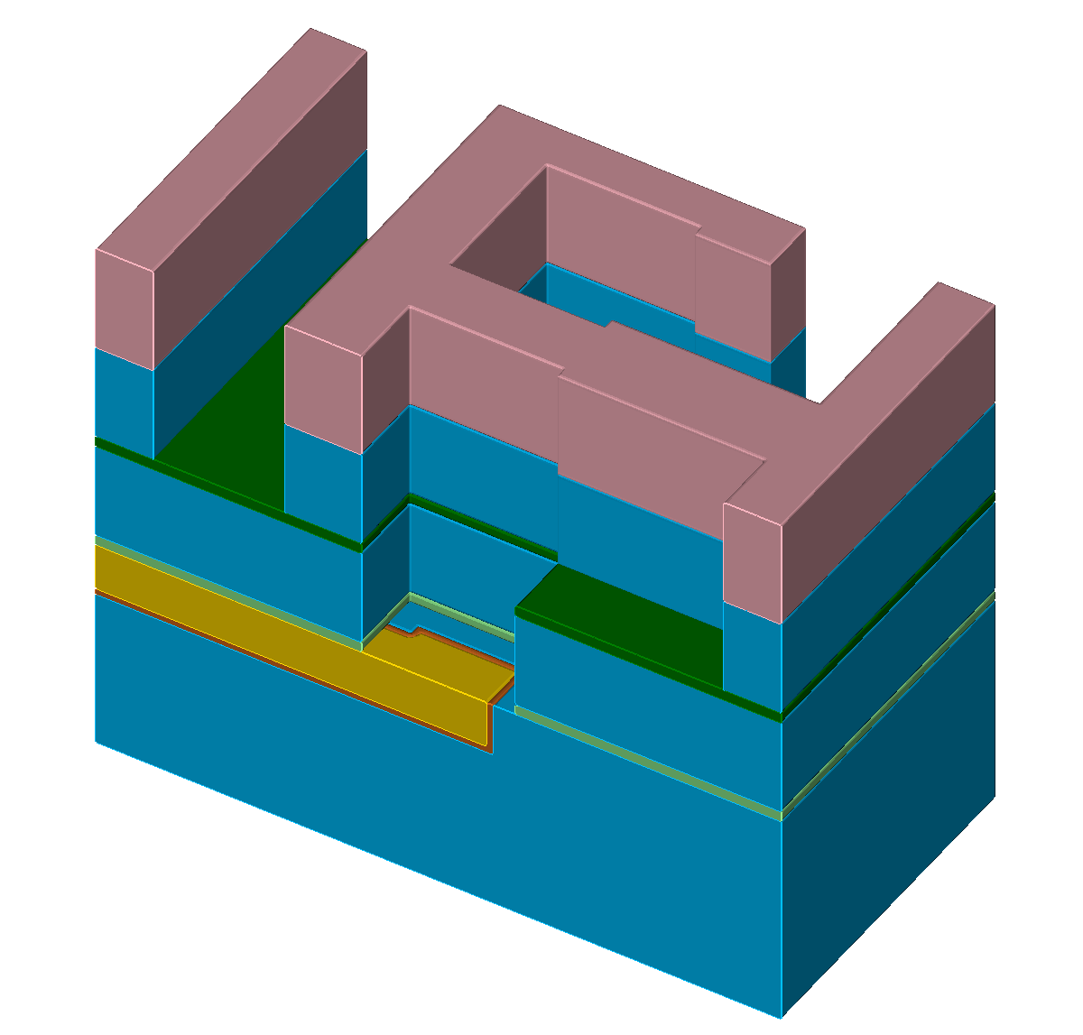
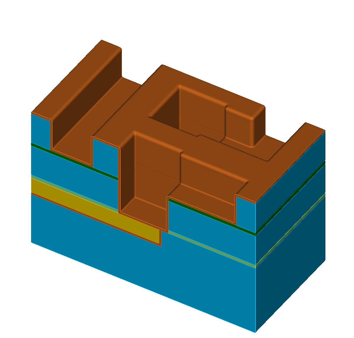
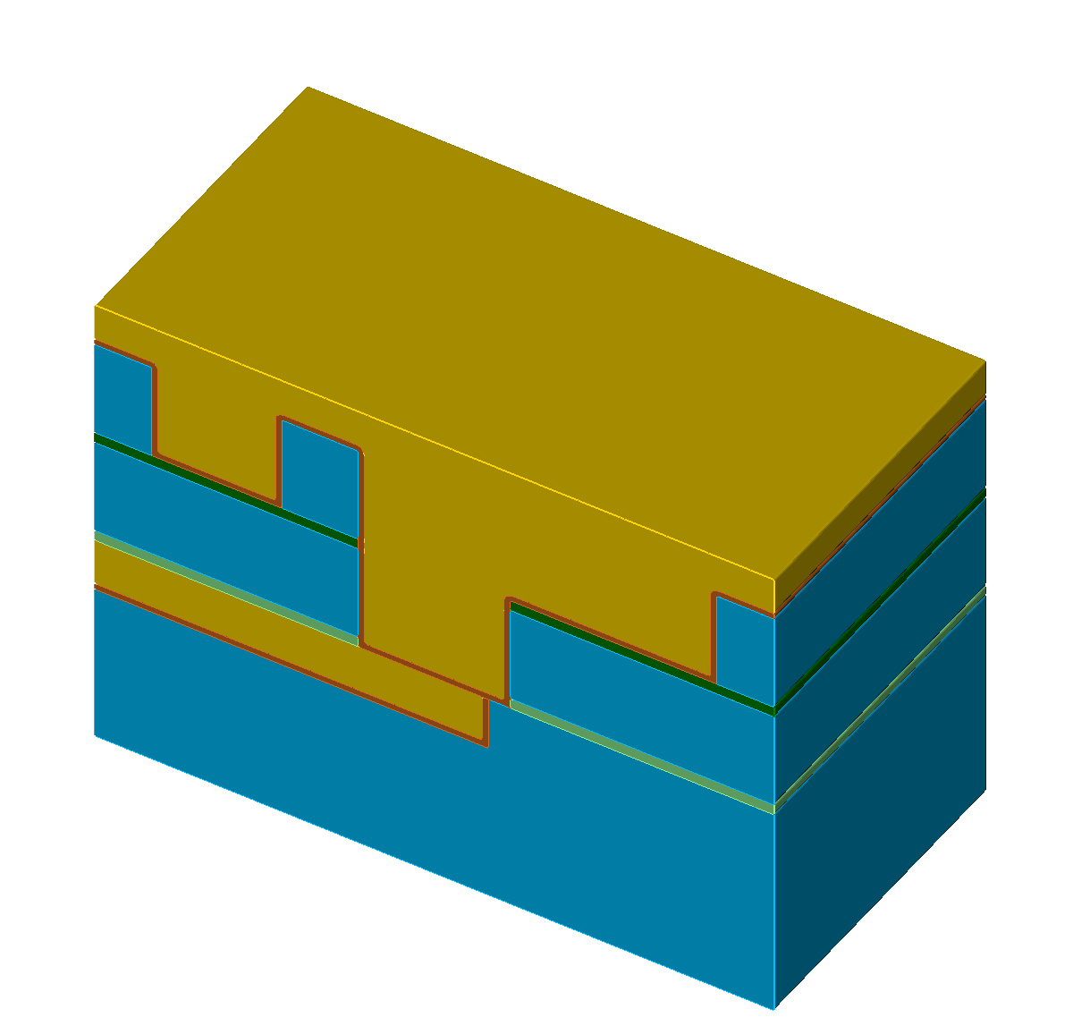
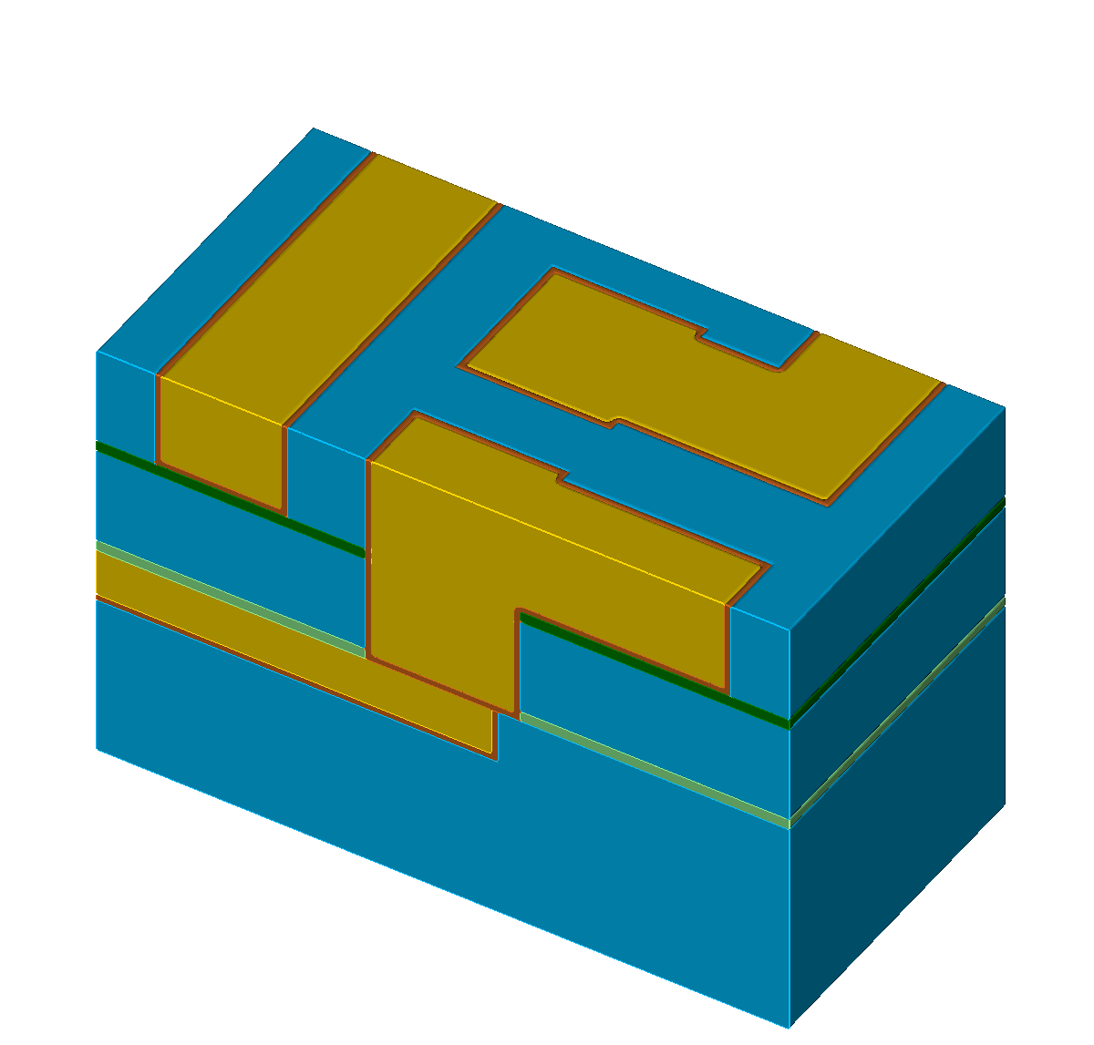
Figure 5.1: Processing steps for the self-aligned Dual-Damascene process. The material legend is shown in (a). Figures (b) to (l) illustrate all processing steps to create a metalization layer on top of an existing metalization layer (the square domain is clipped along one axis for better visibility). First row (b) to (c): Initial patterned planar conductor and deposition of three layers: A diffusion barrier, a dielectric material, and an etch stop material. Second row (d) to (f): Patterning of the etch stop layer (at the position of the vias) including the deposition of the second dielectric layer. Third row (g) to (i): Patterning of the dielectric layers (vias and lines) including opening of the diffusion barrier layer around at the position of the via. Last row (j) to (l): Copper metalization including the deposition of a metal seed layer and chemical-mechanical planarization after the copper deposition.
5.3 Multi-Material Representation
The main focus of this work is the extension of a single-material simulation framework [202] to support multi-material simulations. This extended framework is subsequently used to investigate computationally efficient methods for flux calculation applied to 3D etching and deposition processes, i.e., the iterative partitioning method introduced in Section 5.4 [17]. The original single-material framework is based on the sparse volume data structure implemented in OpenVDB [223], [224] and utilizes the provided methods for surface advection and extraction. All described advection steps are performed using an implicit level-set representation of the surface [204]. An explicit surface representation is only used for the flux calculation step. It is extracted from the level-set using OpenVDB’s volumeToMesh routine, which results in a quad-based surface mesh. Hence, each quad has to be split in order to obtain a triangulated surface mesh. This is achieved by subdividing the quads into two triangles depending on the distance to the zero-level-set as guidance for the subdivision template. The actual ray-surface intersection tests are conducted using Embree [225].
The single steps comprising the original flux calculation method in [202] are discussed in detail below and will act as starting point for the discussion of the implemented extensions to obtain an improved multi-material iterative partitioning scheme [17]. Originally, each timestep of the etching simulation consists of the following main computational tasks: (a) computing the flux rates on the surface, (b) evaluation of the normal surface velocity \(V_n\), and (c) the surface advection step. The normal surface velocity \(V_n\) occurring in etching simulations depends on the flux rates \(R\) of the involved particle types
\( \seteqsection {5} \)
\begin{equation} V_n(\mathbf {x}) = f(R_1, R_2, ..., R_k). \end{equation}
Here, \(k\) denotes the number of considered different particle types. Furthermore, the flux rates depend directly on the incoming flux distribution \(\Gamma _\text {in}\). Weighing all incoming directions for \(\Gamma _\text {in}\) equally yields
\( \seteqsection {5} \) \( \seteqnumber {2} \)
\begin{equation} R(\mathbf {x}) = \int _\Omega \Gamma _{in}(\mathbf {x}, \boldsymbol {\omega }_{d\Omega }) d\Omega \ , \end{equation}
where \(\boldsymbol {\omega }\) represents the incoming direction, whereas \(\Omega \) is the upper hemisphere facing the source plane. In the original single-material framework, \(\Omega \) is discretized using a subdivided icosahedron [202]. This discretization plays a key role in the surface visibility calculations, where for each triangular surface element its visibility to the source is tested, using the centroids of the mesh elements as starting points. Finally, a numerical integration over the visible solid angles for all directions using a centroid rule is conducted [218].
In a multi-material simulation a straightforward way would be to represent each material region using a dedicated level-set function (see Figure 5.2a). In the advection phase, each material region would have to be advected separately, potentially resulting in mutual intersections. In such cases, the parts of a material region which are intersected by another material region would have to be treated as inactive and not be advected. To solve this issue, one option would be to utilize Boolean operations between the material regions to dissolve the intersections. However, this approach requires an algorithm deciding which material fills the former intersected volume.
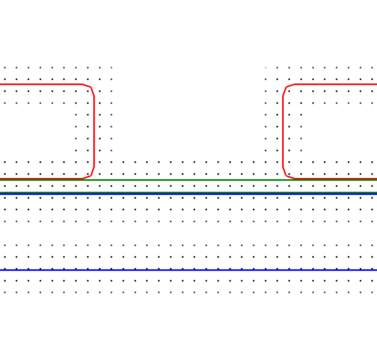
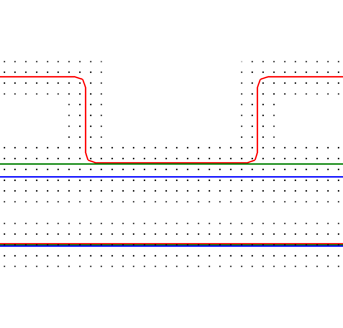
Figure 5.2: An exemplary multi-material stack comprised of a thick region at the bottom (blue), a thin layer (green), and a red top layer (red). (a) Depicts a cross section of the material regions showing the grid points of the level-sets and the extracted level-sets in color. (b) The additive level-sets scheme from bottom to top (blue, green, and red).
The presented extension in this work is based on a total union of all regions, similar to ideas proposed in [226], [227]. Subsequently, the advection of the surface is conducted using the top layer shown in Figure 5.2b. However, determining the correct surface speed of the underlying material is not a trivial task, since it is necessary to detect the active material for each point comprising the top layer. In order to obtain this information, for every point \(\mathbf {x}\) the active material is determined by iterating the values of all level-sets stored in \(\mathbf {x}\). Eventually, the level-set with the smallest value in the point is considered to be the active material’s level-set. Nevertheless, it can happen that two level-sets have the same minimum value. To resolve such a case, the materials are always checked in a fixed order and the lower level-set is chosen as active material if identical values are found. Afterwards, the etching is performed by advecting the top layer and transferring the information about removed material to all underlying level-sets using Boolean operations between the top layer and each material region’s level-set. This top layer method has a major advantage as material layers can be modeled with sub-grid resolution if the level-sets for the different materials are modeled in a way that they do not directly map to the material regions, but are constructed additively.
With this top layer advection method, the development of a material stack utilizing also sub-grid resolution layers during the etching process is schematically depicted in Figure 5.3. In the beginning of the etching step (Figure 5.3a), three different material regions are present (red, green, blue). During the etching with the subsequent advection of the top layer, the green layer is etched first into sub-grid resolution (Figure 5.3b), and finally fully etched away in the left part of the schematic (Figure 5.3c). When a region of a material layer is fully etched away (green) and subsequently the underlying material (blue) becomes active, the surface velocities of all involved materials have to be averaged. This is necessary, since if only a single surface velocity would be considered, e.g., only the green layer, wrong surface advection speeds would be computed.

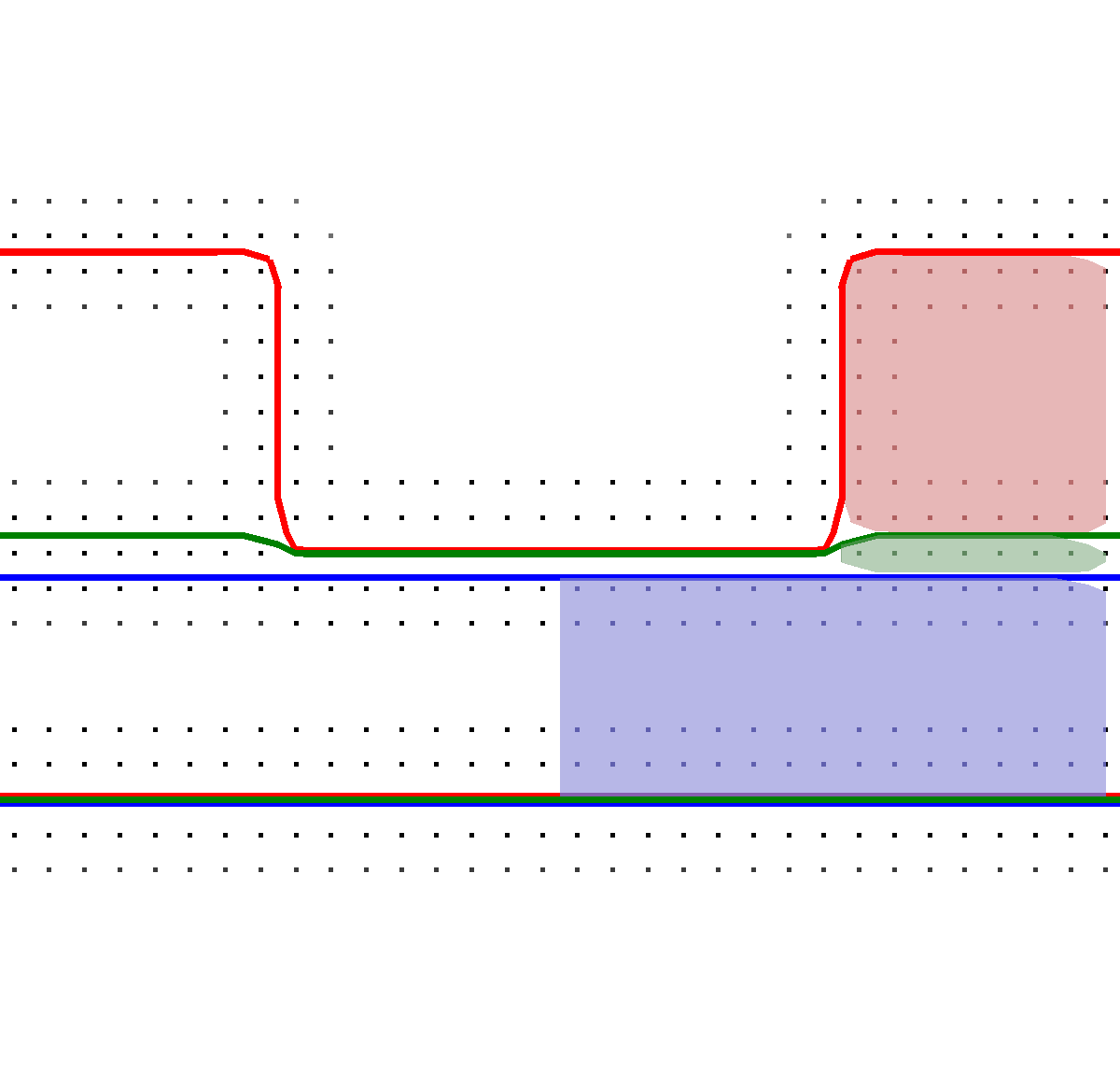
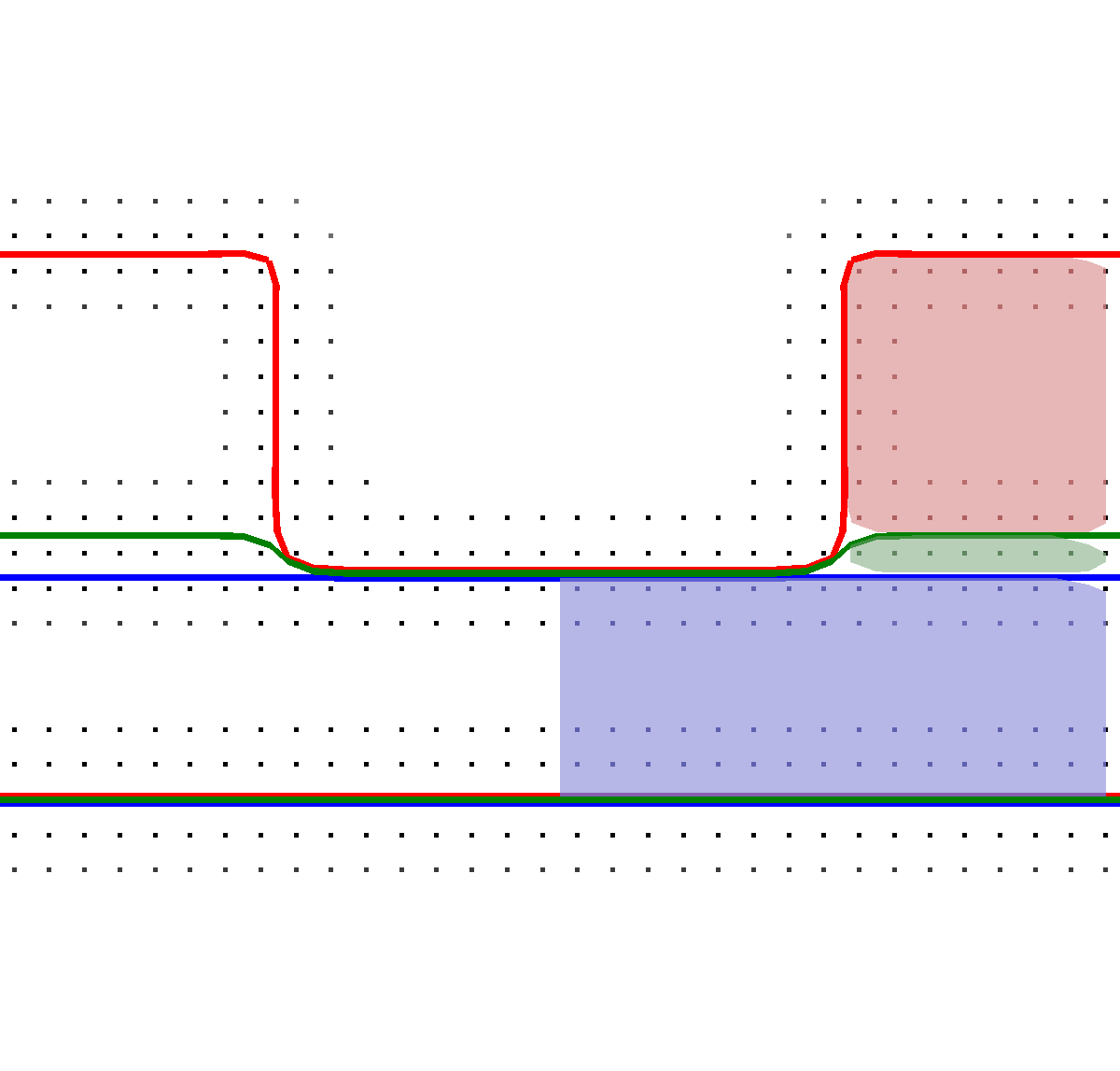
Figure 5.3: The multi-material schematic process according to Figure 5.2 is shown. (a) Start of the etching process. (b) The green layer in sub-grid resolution. (c) Finally, the green layer is fully etched.
5.4 Multi-Material Interface-Aware Iterative Partitioning
To derive further key extensions required for the single-material framework to handle multi-material simulations, a brief overview of the original flux rate calculation approach presented in [202] is given. The main idea is based on the selection of a suitable subset (sparse set) of the triangular mesh elements representing the surface, which thus can be seen as a partitioning of the surface mesh similar to mesh coarsening approaches [56], [58]. However, no topological operations on the mesh elements themselves have to be conducted. The sparse set drastically reduces the necessary integration points required in the flux calculation step. The creation of the sparse set is initialized by a random selection of triangular surface mesh elements with a fixed edge distance \(d_\text {max}\), ensuring a balanced distribution of mesh elements in the sparse set. \(d_\text {max}\) is the number of mesh edges to be crossed from one selected triangular surface mesh element to another (see Definition 2.1.3). The iterative partitioning scheme introduced in [202] is used to refine the initial sparse set obeying two refinement conditions between two adjacent sparse points: A threshold for the flux difference and a threshold for the difference of the normal angles. The idea behind the latter is that a large difference in normal angles denotes important geometrical features which have to be captured and preserved throughout a simulation. Similarly, the flux difference threshold ensures that the gradient of the flux between neighboring selected sparse points yields a smooth distribution of flux rate values over the simulation domain. Finally, the computed flux rate using the sparse set is extrapolated constantly to the surrounding adjacent mesh elements and smoothed utilizing a diffusion approach.
From a computational point of view, the flux calculation algorithm based on the sparse set consists of four main tasks: (1) the initial creation of the sparse set ensuring a fixed edge distance of \(d_\text {max}\) between adjacent sparse points, (2) computing the flux rates for the initial sparse set, (3) the refinement of the initial sparse set obeying the refinement conditions, and (4) the computation of the flux rates for the newly added points to the sparse set. An iterative execution of steps (3) and (4) is conducted until a minimum distance between adjacent points in the sparse set is obtained.
The aforementioned refinement condition based on flux and normal angle thresholds is also applied in the developed multi-material iterative partitioning method in order to evaluate the flux rates for the sparse set. Thus, the maximal normal deviation \(v_\text {max}\), the average flux difference \(u_\text {avg}\), and the maximum flux difference \(u_\text {max}\) are used to define the thresholds for the normal angle deviation \(t_\text {angle}\) and the flux difference \(t_\text {flux}\). These thresholds form the refinement condition \(RC(i)\) for a surface point \(i\) of the sparse set used in the present work:
\( \seteqsection {5} \) \( \seteqnumber {3} \)
\begin{equation} {\text {$RC$}}(i)= \begin {cases} true, & \text {if } \ u_{max_i}> t_\text {angle}, \\ true, & \text {if } \frac {u_{avg_i} + u_{max_i}}{2}> t_\text {flux}, \\ false, & \text {otherwise.} \end {cases} \label {equ:flux:refcon} \end{equation}
The definition of \(RC(i)\) is specifically designed to capture the geometric features as well as the high gradients occurring in the etching simulation using a Dual-Damascene geometry. Different simulation geometries, however, potentially require a different refinement condition to create a suitable sparse set capturing the flux rates in the relevant regions.
Although the refinement condition \(RC(i)\) is modeled such that the geometrical features and flux gradients are captured properly, it has to be ensured that the potentially highly different surface velocities of the different materials in a multi-material simulation are considered appropriately. Thus, the iterative partitioning scheme introduced in [202] is extended, such that mesh cells on the top layer forming a material interface are added to the sparse set by setting their maximally allowed edge distance to \(d_\text {max}=0\). An exemplary partitioning considering material interfaces is depicted in Figure 5.4, where all mesh cells forming the material interface are present in the sparse set. Therefore, a high density of surface cells in material interface regions is guaranteed ensuring correct calculation of the surface flux rates for the different materials.


Figure 5.4: Top layer across a material interface (dotted line). Sparse set cells are labeled with 0, while the cells forming the surrounding patch are labeled with their distance to the sparse set. Solid black lines denote the connection between the cells of the sparse set. (a) the region is partitioned into two patches (red and blue) using \(d_\text {max}=8\), omitting material information; (b) material interface-aware partitioning using \(d_\text {max}=0\) for cells embedding the material interface: The green cells, which are part of the sparse set, follow the material interface and allow for a proper representation.
5.5 Evaluation
The evaluation of the introduced multi-material interface-aware partitioning method is conducted using BP1 and utilizing a typical etching simulation occurring in Process TCAD, i.e., the etching step shown in Figures 5.1g-5.1h. A particular focus is on the computational performance, i.e., the strong scaling capabilities, of the etching simulation with the sparse set approach. Additionally, the accuracy of the presented partitioning method is compared to the conventional approach of evaluating all surface mesh cells (dense approach).
5.5.1 Simulation Setup
An integral part in the etching simulation is the definition of the normal surface velocity \(V_n(\textbf {x})\). For the conducted work \(V_n(\textbf {x})\) is defined as
\( \seteqsection {5} \) \( \seteqnumber {4} \)
\begin{equation} V_n(\textbf {x}) = \alpha (M(\textbf {x}))\cdot R(\textbf {x}) \ , \end{equation}
with \(\alpha \) being a material dependent scalar weighting factor and \(R\) the direct flux incoming from the ion source. Table 5.1 lists the applied weighting factors for the different materials normalized to the weighting factors of the dielectric. These weighting factors are set to arbitrary values for the conducted benchmarks in order to show the ability of the presented multi-material simulation approach to handle highly different surface reaction behaviors. Hence, the weighting factors for both, the etch stop and the diffusion barrier, are set to equal values of \(\alpha =0.02\). Similarly, the copper layer and the metal seed layer are assigned equal factors of \(\alpha =0.1\). The actual simulation geometry used within this study is shown in Figure 5.5.
| Material \(M\) | Weighting Factor \(\alpha \) | |
| Hard Mask | 0.01 | |
| Dielectric | 1.0 | |
| Etch Stop | 0.02 | |
| Diffusion Barrier | 0.02 | |
| Copper | 0.1 | |
| Metal Seed | 0.1 | |
Table 5.1: Colors and normalized weighting factors corresponding to the different etch rates for the materials used in the etching simulation in Figure 5.5.
For the creation of the sparse set \(d_\text {max}=32\) is applied for all conducted simulations, yielding a total number of six iterations for the partitioning methods. The number of iterations for the smoothing of the extrapolated constant values is fixed to \(d_\text {max}/ 4 = 8\). Due to these specific choices a trade-off between accuracy of the flux calculation and maximal approximation of the surface using the sparse set is achieved for the Dual-Damascene etching process.
The highly focused ion source applied in the simulation is modeled using a power cosine function with an exponent of \(n=1000\), which is a popular choice for modeling accelerated ions in Process TCAD [218]. For the sake of simplicity only the direct flux is considered in the conducted simulations. As already mentioned above, a subdivided icosahedron approach is used with the subdivision parameter set to 5 in order to limit the influence of the integration accuracy, following the results in [218].
The evaluated resolutions of the underlying level-sets range from 32 to 128 cells per unit length yielding 140 to 560 timesteps and covering lower as well as higher mesh resolutions. This allows for an evaluation of the effects of different level-set resolutions on the simulation accuracy. As the timesteps for all resolutions cover an identical simulation timeframe (i.e., \(T=2.0\)), the edge stop layer is reached approximately at \(T\approx 0.5\) and the diffusion barrier at about \(T\approx 1.0\). Table 5.2 summarizes all the level-set parameters.
| Cells | Vertical Cells | Horizontal Cells | Triangles | Vertices | Timesteps |
| 32 | 80 | 96 \(\times \) 96 | 28,642 | 56,384 | 140 |
| 64 | 160 | 192 \(\times \) 192 | 113,986 | 226,176 | 280 |
| 128 | 320 | 384 \(\times \) 384 | 455,298 | 907,008 | 560 |
Table 5.2: The investigated level-set resolutions, i.e., cells per unit length, corresponding initial vertical and horizontal domain resolutions, the number of triangles and vertices in the initial surface mesh, and the number of required timesteps until simulation time reaches \(T=2.0\).
Additionally, the threshold parameters for the refinement condition are varied around their proposed default values (i.e., \(t_\text {angle} = 0.1\) and \(t_\text {flux} = 10\)) as described in [202]. This enables the evaluation of their influence on both, accuracy and computational performance, of the flux calculation step. For the normal angle threshold \(t_\text {angle}\) between two points of the sparse set the variations evaluated are: 0.05 and 0.2. The values for the variation of the flux difference threshold are set to 5 and 20% difference to the global maximum of the calculated flux in each timestep.
5.5.2 Performance and Accuracy
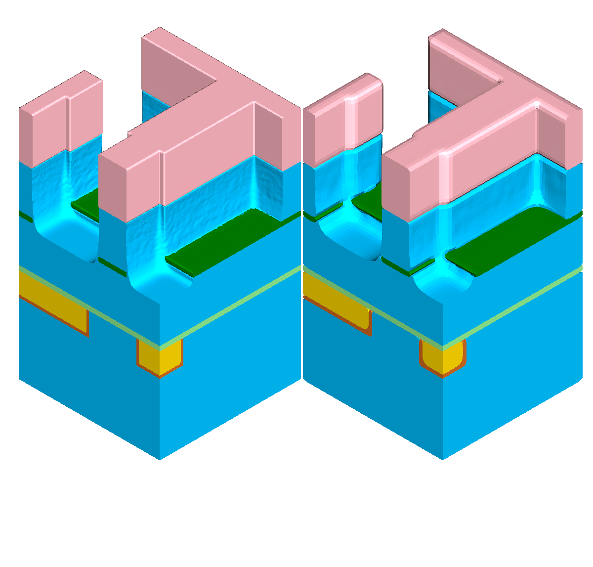
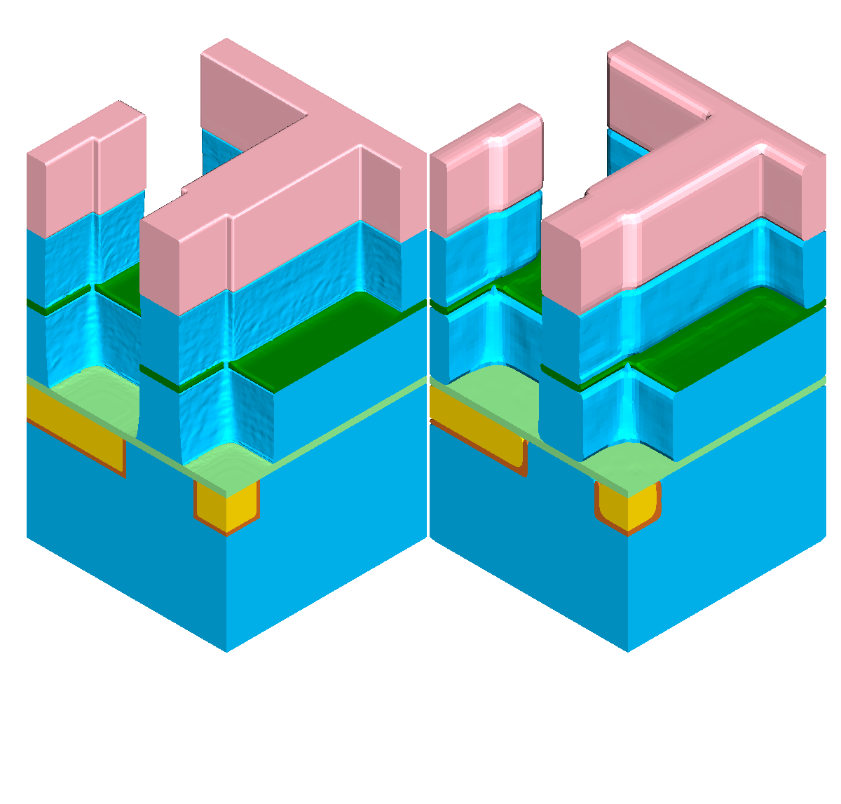
First, the influence of different level-set resolutions on the resulting simulation geometry is briefly discussed. Figure 5.6 depicts the simulation results at different times \(T\) during the simulated etching of the dielectric layer with the left part depicting the highest investigated level-set resolution of 128 cells per unit length and the right part of 32 cells per unit length. The investigated threshold values for the refinement condition defined in Equation 5.3 are set to their proposed default values \(t_\text {flux}=10\) and \(t_\text {angle} = 0.1\). One key aspect of using lower resolutions is the observable rounding of actually sharp geometrical features resulting from the implicit level-set representation. As expected, the influence of the level-set resolution is higher the thinner the material layer is, for example, the etch stop layer experiences more influence than the dielectric layer.

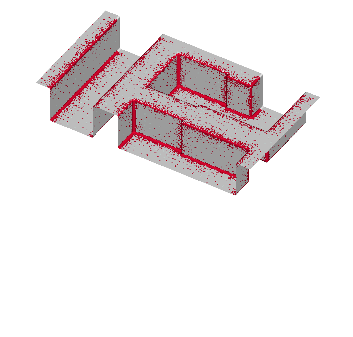
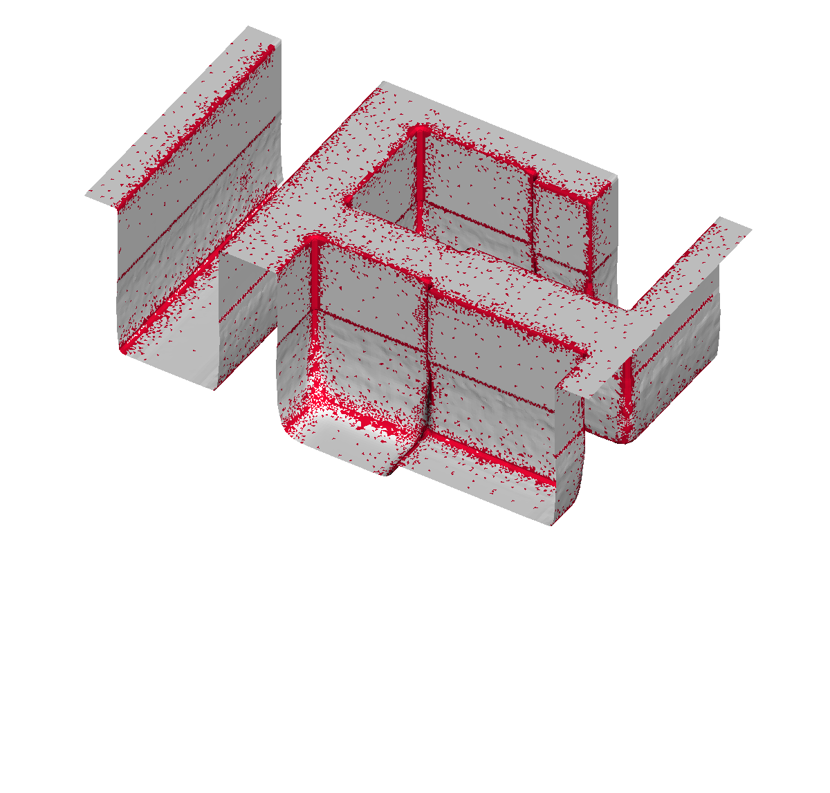
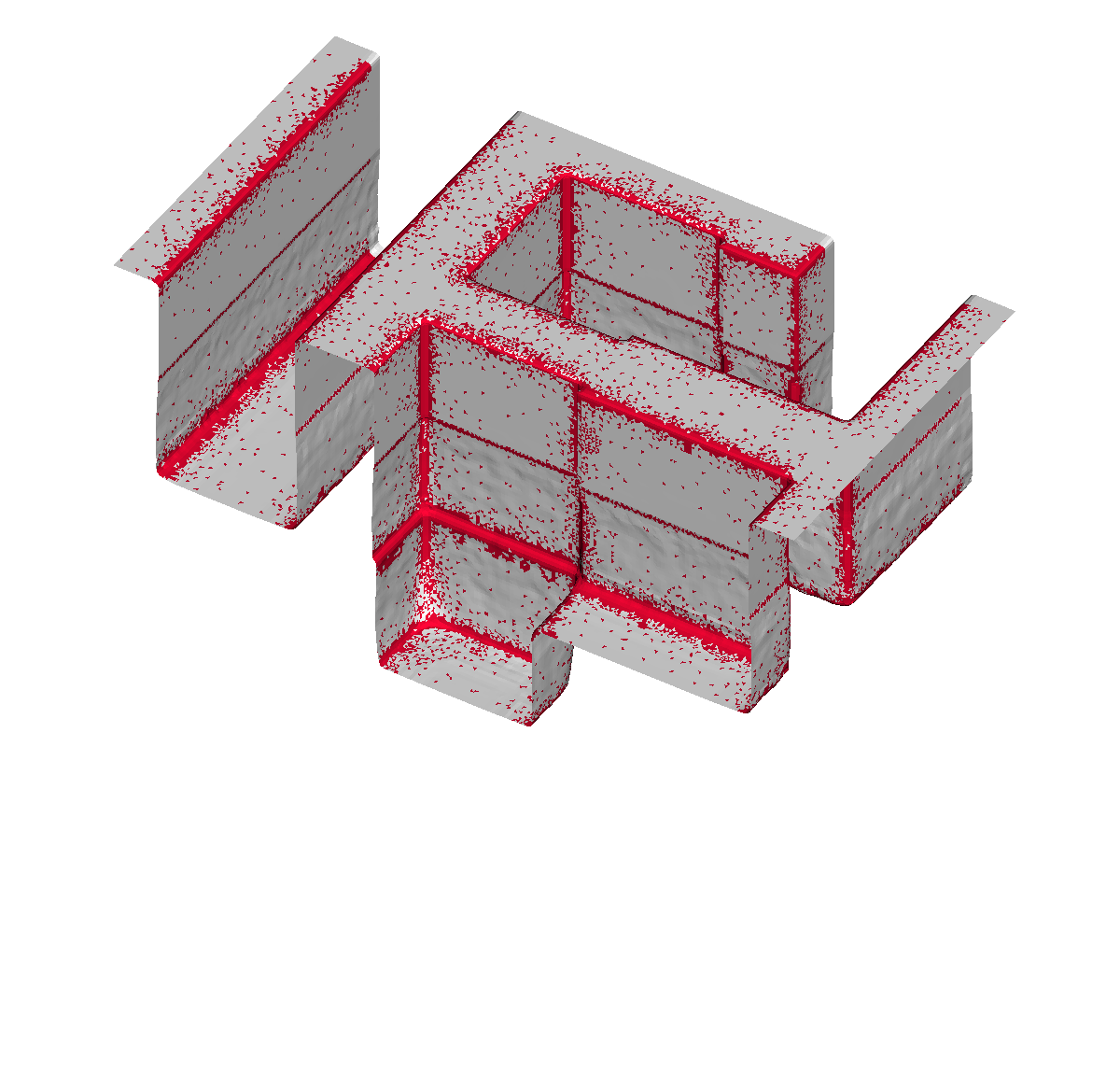
A direct influence on the accuracy of the etching simulation is caused by the selection of the cells for the sparse set, particularly for sharp geometrical features. To prove that the designed refinement condition \(RC(i)\) captures the geometrical features properly, Figure 5.7 shows the created sparse sets using a level-set resolution of 64. As intended, the density of the sparse cells increases towards sharp geometrical features but also in regions where high flux gradients are computed. Furthermore, since the surface mesh cells forming a material interface are forced to be contained in the sparse set their density increases around these interfaces. To quantify the reduction of cells to be evaluated, the ratio of the number of cells used for the dense approach to the number of cells selected for the sparse set is used:
\( \seteqsection {5} \) \( \seteqnumber {5} \)
\begin{equation} x_\text {rel} = \frac {n_{\text {dense}}}{n_{\text {sparse}}} \end{equation}
The introduced ratio \(x_\text {rel}\) can be seen as the theoretical limit for the obtainable relative speedup \(S_\text {rel}\) defined in Equation 5.6. \(S_\text {rel}\) denotes the ratio of the flux calculation runtime of the dense approach over the flux calculation runtime using the sparse set and must not be confused with the conventional speedup obtained by parallelization defined in Equation 2.23:
\( \seteqsection {5} \) \( \seteqnumber {6} \)
\begin{equation} S_{rel}=\frac {\text {t}_{\text {dense}}^{\text {flux}} } {\text {t}_{\text {sparse}}^{\text {flux}}} \label {eq:flux:speedup} \end{equation}
Naturally, when introducing an approximation method, one key aspect is to asses its accuracy compared to a standard approach. Thus, the differences of the surface positions between the approach based on the sparse set and the dense approach are computed for fixed timestep intervals. Throughout the simulations, a constant Courant–Friedrichs–Lewy (CFL) number of \(\alpha _{CFL} = 0.4\) is used [228]. The accuracy of the sparse set method is evaluated by calculating the closest distance, i.e., surface deviation, for each surface point between the surface meshes resulting from the dense and the sparse method.
Figure 5.8 plots the relative cell factors \(x_\text {rel}\), the obtained relative speedups \(S_\text {rel}\), and the maximum computed surface deviations for three different level-set resolutions (32, 64, and 128). Using the presented sparse set method the obtained relative speedups for a level-set resolution of 32 range from 1.9 to 2.5, being about 46% below the maximum theoretical limit of \(x_\text {rel}=4.6\) (Figure 5.8a). As expected, Figures 5.8b-5.8c prove that the relative speedup increases with higher level-set resolutions. For resolution 64 the speedups range from 2.8 to 4.4 with \(x_\text {rel}\) having a maximum value of 7.7, whereas for resolution 128 the achieved relative speedups range from 4.1, to 7.0 with a peak of \(x_\text {rel}\) at 14.6. Obviously, the observed gap between the relative speedups \(S_\text {rel}\) and their upper theoretical bound \(x_\text {rel}\) is caused by the computational overhead induced by the creation of the sparse set (Section 5.5.4 will elaborate on this topic). In addition to the relative speedups, Table 5.3 contains the recorded overall runtimes for the dense and sparse evaluation approach for the investigated level-set resolutions. However, for the presented approach only the flux calculation steps are parallelized in contrast to the serial initial creation step of the sparse set and its subsequent refinement (see Section 5.4). Therefore, the runtimes show that the serial parts are jeopardizing the maximum obtainable speedup, e.g., about 3.8 for the highest resolution compared to the maximum peak of \(S_{rel}\) of about 14.6.
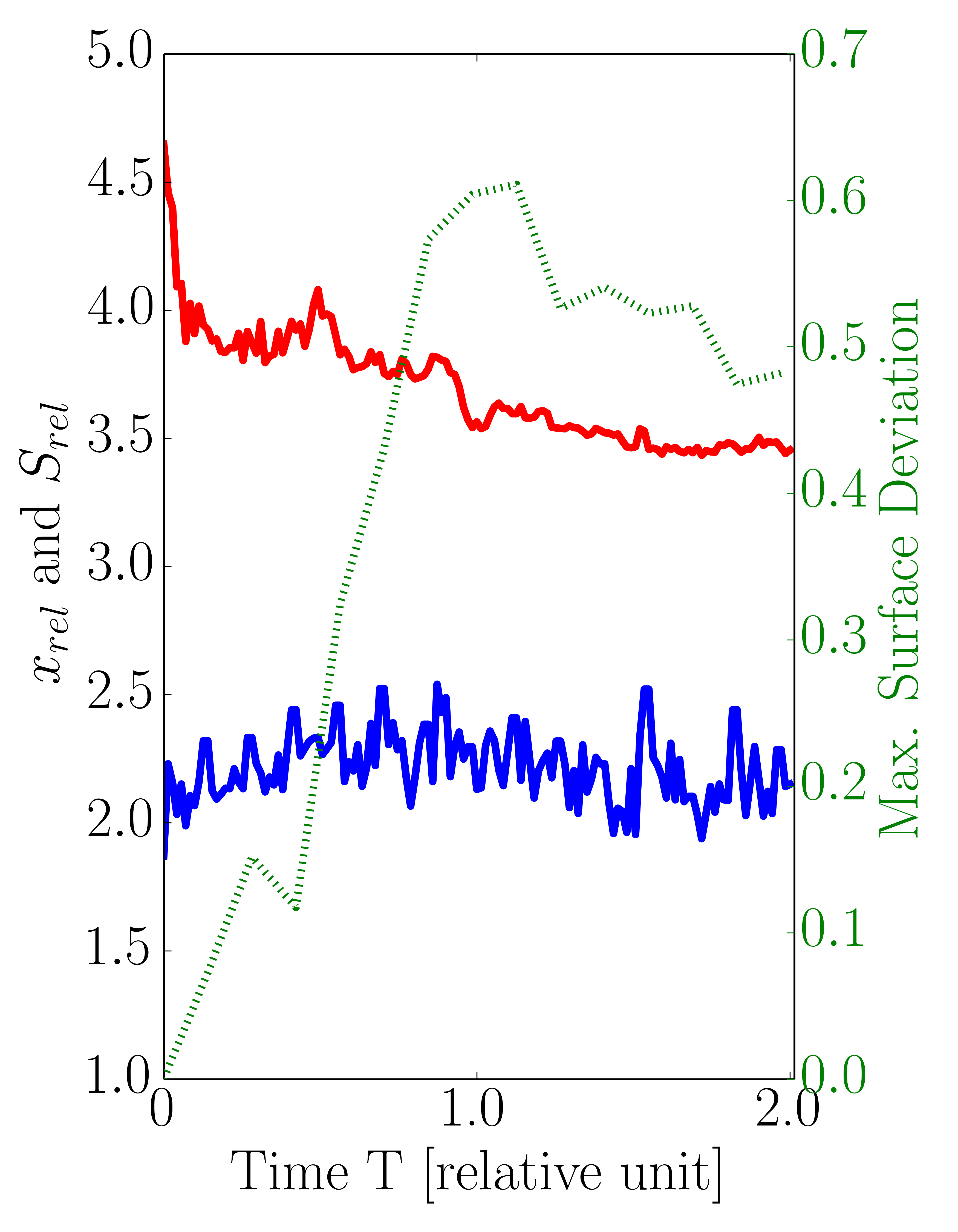
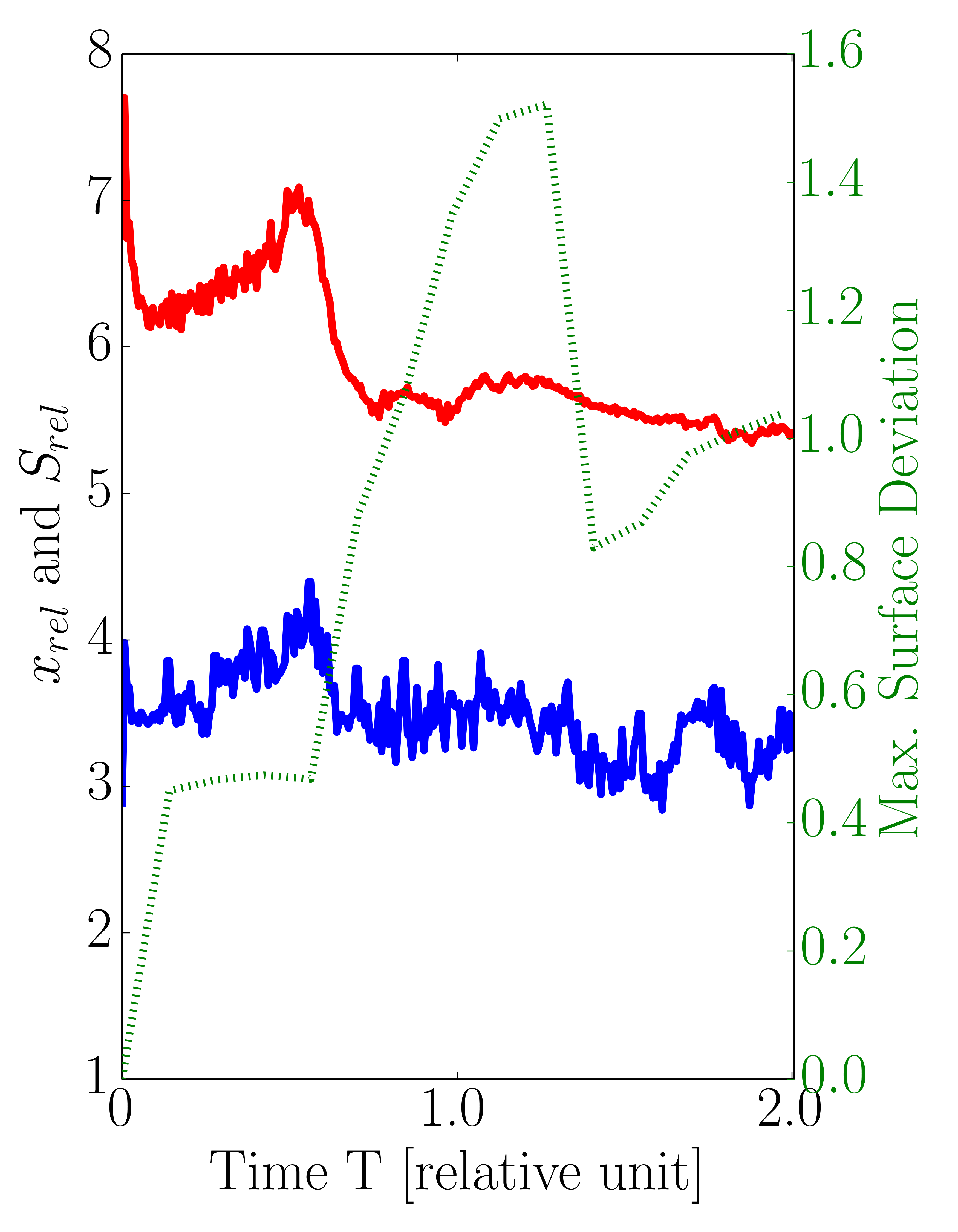
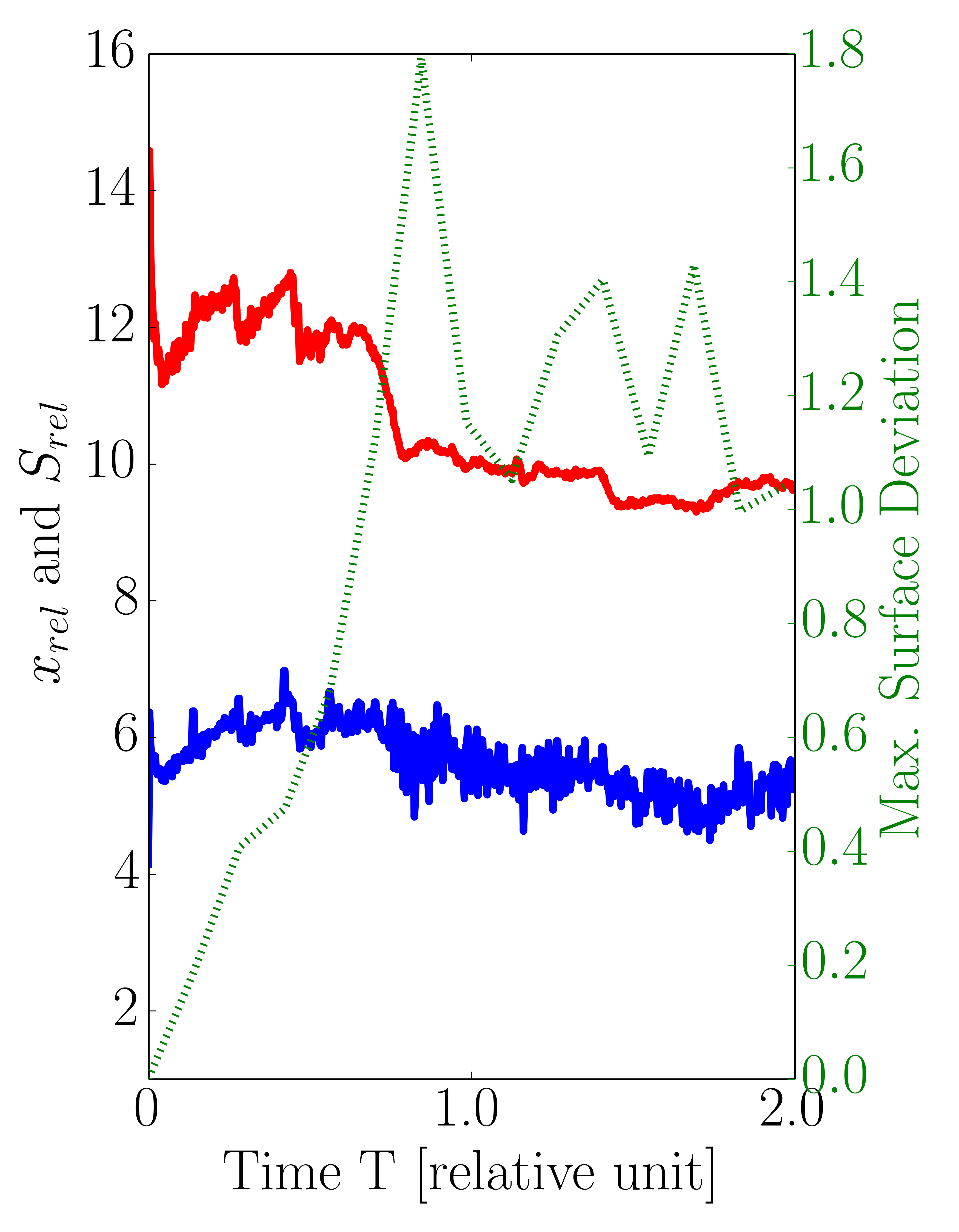
Figure 5.8: Ratio between dense and sparse number of cells \(x_\text {rel}\), relative speedup \(S_{rel}\), and maximum surface deviation (Dev) for level-set resolution of (a) 32, (b) 64, and (c) 128 using the default values for both refinement conditions (\(t_\text {flux}= 10\) and \(t_\text {angle}= 0.1\)). The average values of \(x_\text {rel}\) and \(S_{rel}\) are depicted in Figure 5.9.
| Resolution | Runtime Dense [min] | Runtime Sparse [min] |
| 32 | 22 | 12 |
| 64 | 159 | 60 |
| 128 | 1 209 | 311 |
Table 5.3: Total simulation runtimes in minutes for different level-set resolutions using the dense and sparse approach with the maximum number of 16 threads on BP1.
The results plotted in Figure 5.8 show also the maximum surface deviations between the dense and the sparse approach recorded for the different level-set resolutions: With the highest resolution of 128, the maximum deviation is below 1.8 grid cells corresponding to 0.6% of the via size. For the resolutions 32 and 64 the deviation’s upper bound is 0.7 and 1.6, respectively. These deviations were recorded in the vias, where they correspond to about 3% of the size of the via for resolution 32 and about 1.1% for resolution 64. For all three resolutions the peak of the maximum surface deviations occur around \(T=1.0\). At this timestep of the simulations, the etching process reaches the bottom of the via, i.e., diffusion barrier, and thus the vertical surface velocities in the dielectric disappear. Hence, the maximum surface deviations remain more or less stable for simulation times \(T > 1.0\). The results show that the developed sparse set approach yields superior runtimes for the flux calculation step for all resolutions, while simultaneously producing similar results compared to the dense approach.
5.5.3 Variation of Thresholds
The results presented in this section form the basis for evaluating the sensitivity of the proposed sparse set method with respect to different threshold values for the refinement condition \(RC(i)\) defined in Equation 5.3. For the three different level-set resolutions (32, 64, and 128) the average relative speedup \(S_\text {rel}^\text {avg}\) and the average \(x_\text {rel}^\text {avg}\) are depicted in Figure 5.9 using the threshold variations described in Section 5.5.1.

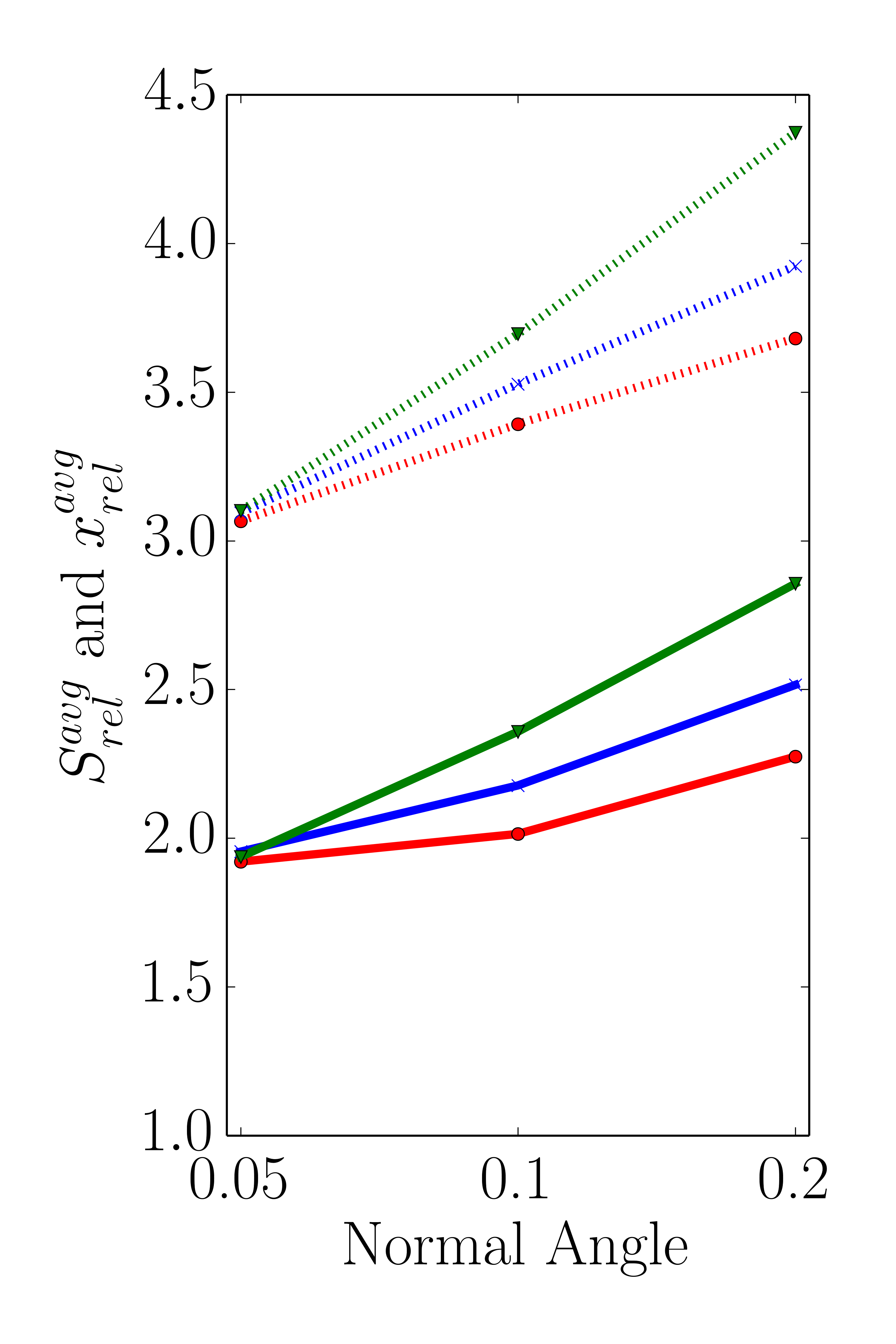
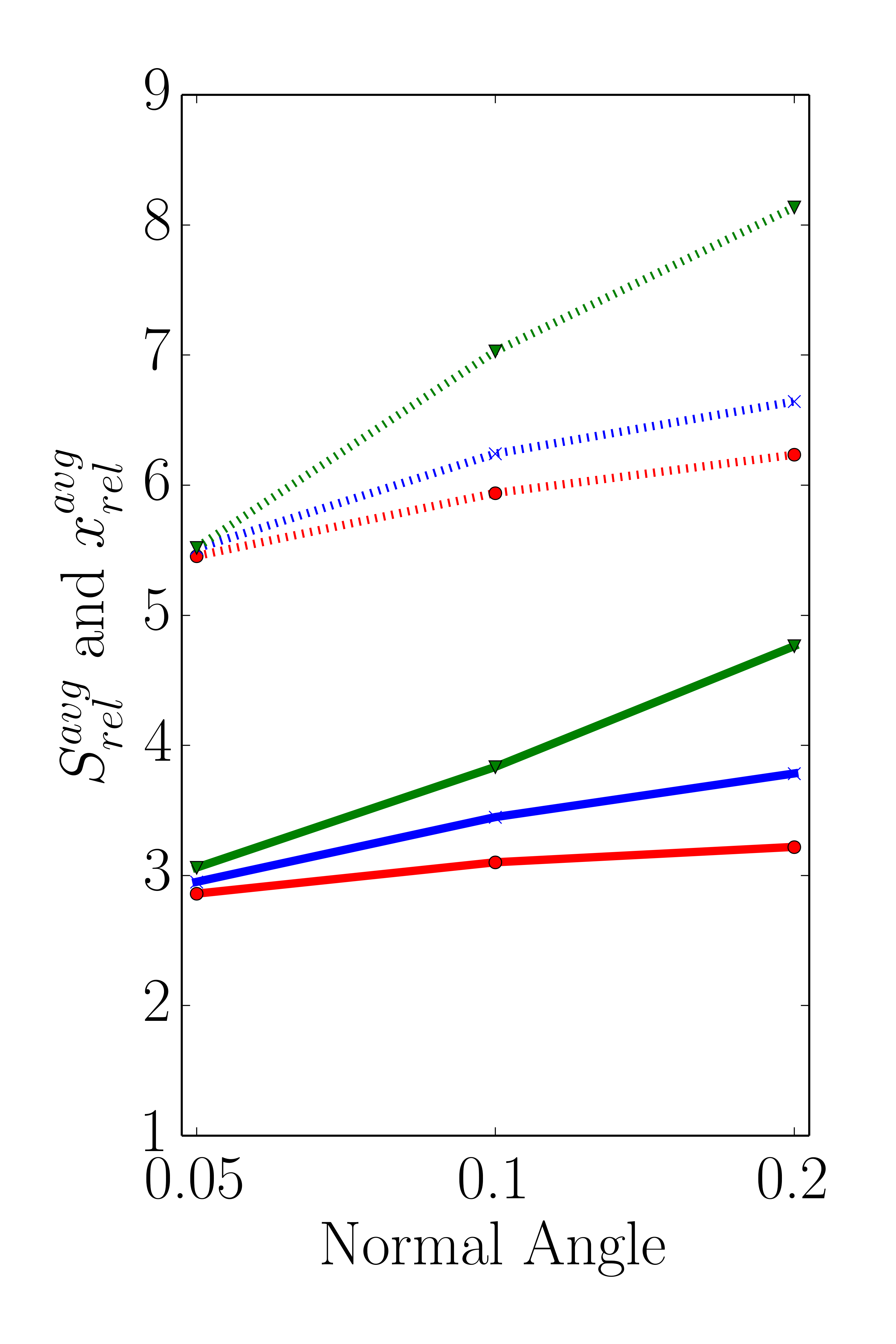

The obtained results for the lowest of the three different level-set resolutions presented in Figure 5.9a prove that the factor \(x_\text {rel}\) increases with both, increasing normal angle and flux angle threshold values. The highest influence is observed for \(t_\text {flux} = 20\). This behavior is caused by the definition of the refinement condition (Equation 5.3): A point is added to the sparse set if either the flux rate threshold or the normal angle threshold is violated. Hence, higher threshold values for the flux rate or the normal angle yield a smaller number of points added to the sparse set. This behavior is also observed for the other two level-set resolutions, 64 and 128, shown in Figures 5.9b and 5.9c, respectively. In addition, the already mentioned discrepancy between \(x_\text {rel}\) and \(S_\text {rel}\) indicate the introduced computational overhead by the iterative sparse set creation process.
Regarding the surface deviations between the dense and the sparse evaluation method, the observed influence of varying threshold values is denoted in Table 5.4. For an easier comparison the surface cell deviations are accumulated in bins of size 0.1 ranging from 0.0 to 0.4. The results in Table 5.4 depict the relative population of the respective bin. As expected, increasing threshold values result in increased surface cell deviations as less cells are added to the sparse set increasing the approximation inaccuracies. Additionally, for the lowest level-set resolution of 32 the percentage of surface cells experiencing a deviation above 0.4 is growing from 0.02 to 0.68% for the smallest (\(t_\text {angle}=0.05\), \(t_\text {flux}=5\)) to the highest (\(t_\text {angle}=0.2\), \(t_\text {flux}=20\)) evaluated threshold combinations. A similar increase in the percentage of surface cells with a deviation above 0.4 is recorded for the level-set resolutions of 64 and 128, where the relative populations increased from 0.28 to 3.8% and from 0.27 to 5.62%, respectively. These results indicate that even with a combination of the highest threshold values (yielding the coarsest sparse set), the total deviations of the sparse set method compared to the dense approach are mostly in the sub-cell region. Hence, the absolute number of surface points experiencing deviations larger than cell-size (including the maximum deviations discussed in Section 5.5.2) is limited, but increases with increasing threshold values.
| Resolution 32 | ||||||||||
| Angle | 0.05 | 0.1 | 0.2 | |||||||
| Flux | 5 | 10 | 20 | 5 | 10 | 20 | 5 | 10 | 20 | |
| Deviation | 0.0–0.1 | 98.62 | 98.05 | 98.45 | 94.40 | 93.66 | 89.67 | 91.12 | 86.24 | 81.33 |
| 0.1–0.2 | 1.17 | 1.57 | 1.26 | 4.31 | 4.97 | 8.65 | 5.55 | 7.06 | 10.82 | |
| 0.2–0.3 | 0.15 | 0.22 | 0.18 | 1.10 | 1.27 | 1.49 | 2.37 | 3.37 | 4.84 | |
| 0.3–0.4 | 0.04 | 0.10 | 0.07 | 0.13 | 0.09 | 0.11 | 0.87 | 2.74 | 2.33 | |
| >0.4 | 0.02 | 0.06 | 0.04 | 0.07 | 0.01 | 0.08 | 0.08 | 0.58 | 0.68 | |
| Resolution 64 | ||||||||||
| Angle | 0.05 | 0.1 | 0.2 | |||||||
| Flux | 5 | 10 | 20 | 5 | 10 | 20 | 5 | 10 | 20 | |
| Deviation | 0.0–0.1 | 96.42 | 92.91 | 92.55 | 96.10 | 89.69 | 85.26 | 95.73 | 88.42 | 80.42 |
| 0.1–0.2 | 2.63 | 5.84 | 6.05 | 2.93 | 7.99 | 8.52 | 3.31 | 9.01 | 9.88 | |
| 0.2–0.3 | 0.46 | 0.71 | 0.80 | 0.51 | 1.67 | 3.14 | 0.51 | 1.88 | 3.76 | |
| 0.3–0.4 | 0.22 | 0.25 | 0.28 | 0.18 | 0.36 | 1.89 | 0.17 | 0.37 | 2.13 | |
| >0.4 | 0.28 | 0.29 | 0.32 | 0.27 | 0.30 | 1.19 | 0.27 | 0.31 | 3.80 | |
| Resolution 128 | ||||||||||
| Angle | 0.05 | 0.1 | 0.2 | |||||||
| Flux | 5 | 10 | 20 | 5 | 10 | 20 | 5 | 10 | 20 | |
| Deviation | 0.0–0.1 | 88.11 | 84.26 | 84.26 | 86.08 | 80.20 | 76.90 | 85.46 | 78.55 | 73.65 |
| 0.1–0.2 | 8.92 | 9.89 | 9.59 | 10.35 | 11.60 | 11.69 | 10.68 | 12.24 | 12.11 | |
| 0.2–0.3 | 2.19 | 3.66 | 3.54 | 2.56 | 4.56 | 4.92 | 2.70 | 5.16 | 5.77 | |
| 0.3–0.4 | 0.50 | 1.38 | 1.57 | 0.68 | 2.13 | 2.26 | 0.76 | 2.26 | 2.86 | |
| >0.4 | 0.27 | 0.81 | 1.04 | 0.32 | 1.51 | 4.23 | 0.40 | 1.79 | 5.62 | |
Table 5.4: Distribution of computed surface deviations (normalized to the cell size) at \(T\approx 1.0\) for different level-set resolutions, normal angle, and flux thresholds. The population of the bins is given in percent.
5.5.4 Strong Scalability
To investigate the strong scaling behavior of both, the dense and the sparse method, the flux calculation runtimes on BP1 are investigated. The thresholds used in the refinement condition for the sparse set creation are set to their proposed default values of \(t_\text {angle}=0.1\) and \(t_\text {flux}=10\).
Both, the average runtimes and the speedups for the dense and the sparse evaluation method, are plotted in Figure 5.10 using dotted and solid lines, respectively. The results show that the flux calculation method based on the sparse set is faster than the conventional dense approach, with the longest runtime difference observed for the highest level-set resolution, i.e., 128. For this resolution, the sparse set method with one and 16 threads outperforms the dense method by a factor of 7.5 and 3.4, respectively. However, for the investigated level-set resolutions the strong scaling with the dense approach is superior to the sparse approach where the difference of the speedups between the two methods increases with increasing level-set resolution. Applying the highest level-set resolution the observed speedup with 16 threads is 26% above the sparse set’s speedup. Furthermore, the sparse set method delivers better results for the lowest level-set resolution regarding its strong scaling capabilities, although the speedup for 16 threads is about 26% below the dense method’s speedup. For level-set resolutions of 64 and 128, the sparse speedup is about 40% and 55% below the dense’s, respectively. Nevertheless, the absolute runtimes of the sparse set method outperform the dense approach. The primary reason for the different runtimes of the two methods is the difference in the number of evaluated surface cells, i.e., the sparse set method uses fewer cells and thus yields better performance for the flux calculation particularly for smaller thread counts.
However, with increasing thread counts the gap between the runtimes of the two approaches decreases due to the serial parts of the iterative partitioning method. This is shown in Figure 5.11, which depicts the different shares of the four main tasks of the flux calculation method introduced in Section 5.4 for a single timestep. The serial case in Figure 5.11a indicates that the used time for the refinement of the sparse set accounts only for 3% of the overall runtimes, whereas the flux calculation for the refined surface cells requires about 87%. Naturally, this changes for 16 threads, as shown in Figure 5.11b, where the share for the refinement step increases ten-fold to about 32%, with the flux calculation of the refined cells decreasing by nearly a third to about 56%. As expected, the results in Figure 5.11 show that the bottleneck of the total process is caused by the serial iterative refinement step for the sparse set. Therefore, the strong scaling of the sparse set is limited due to Amdahl’s law (Equation 2.23). Hence, investigating parallelization approaches for these serial parts would yield a further performance increase. Nevertheless, the presented iterative partitioning method based on the sparse set is able to significantly outperform the conventional method.

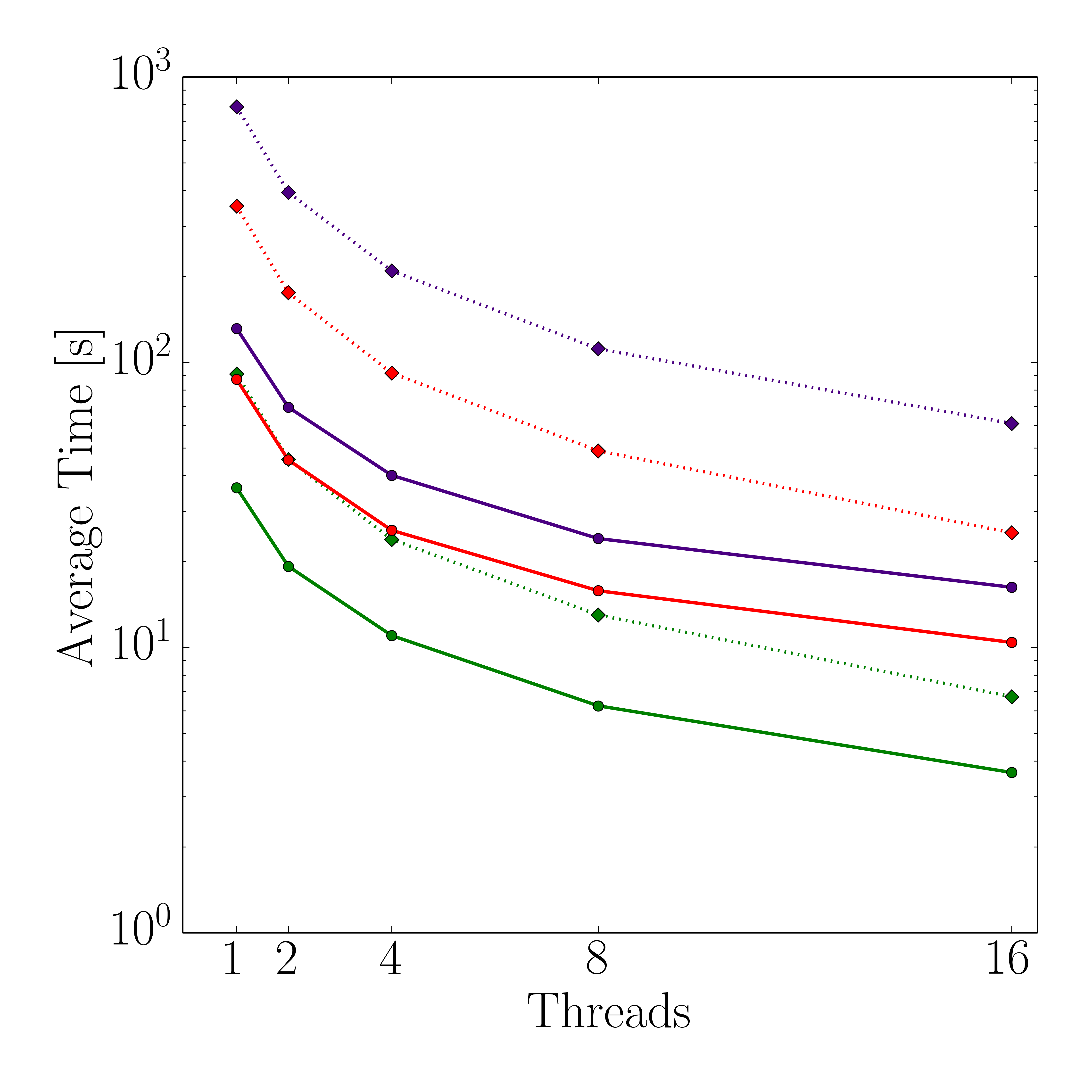
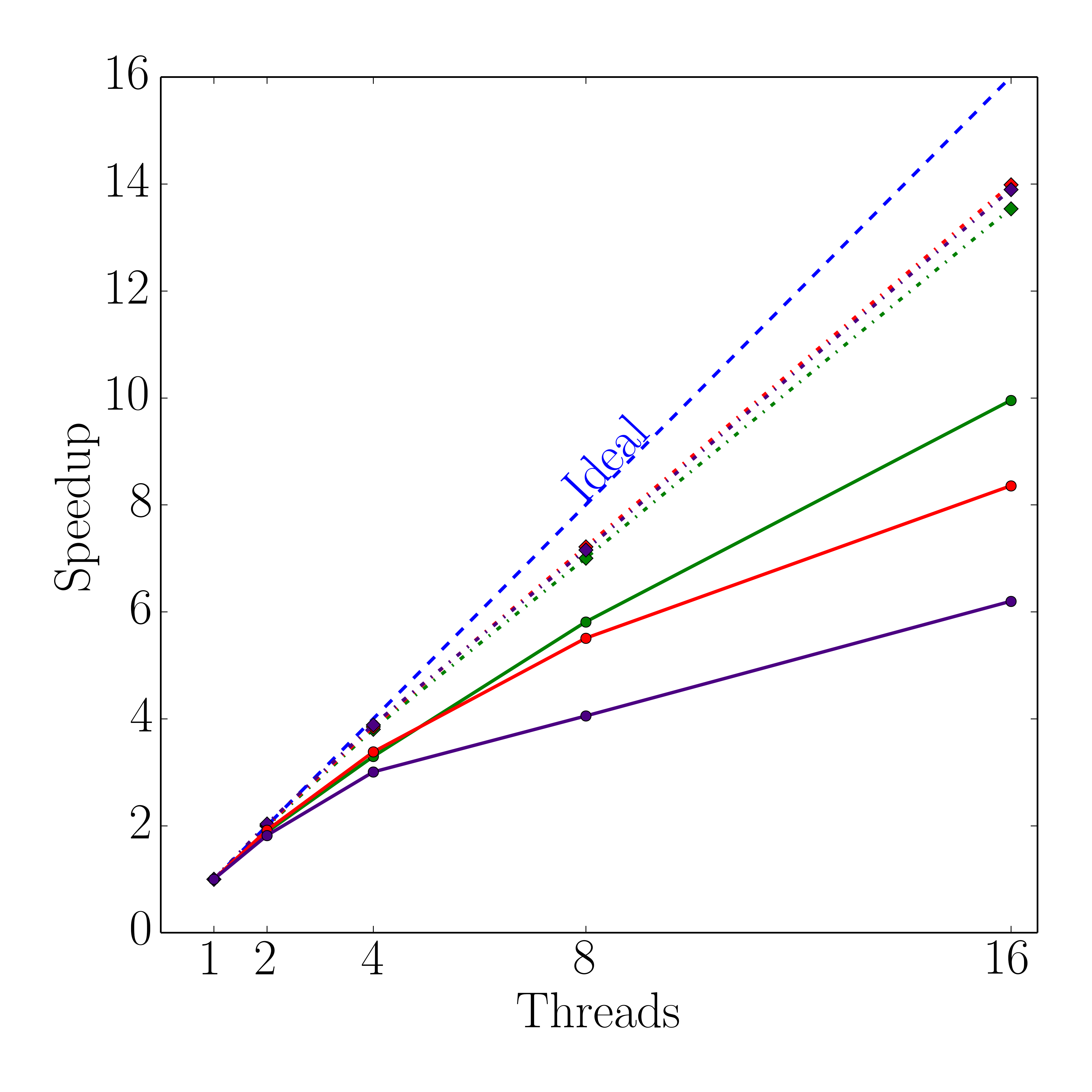

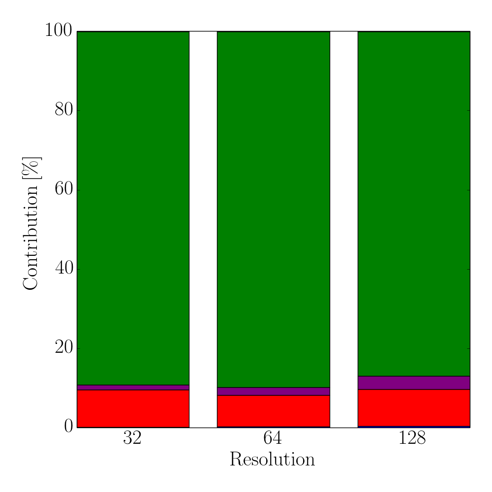
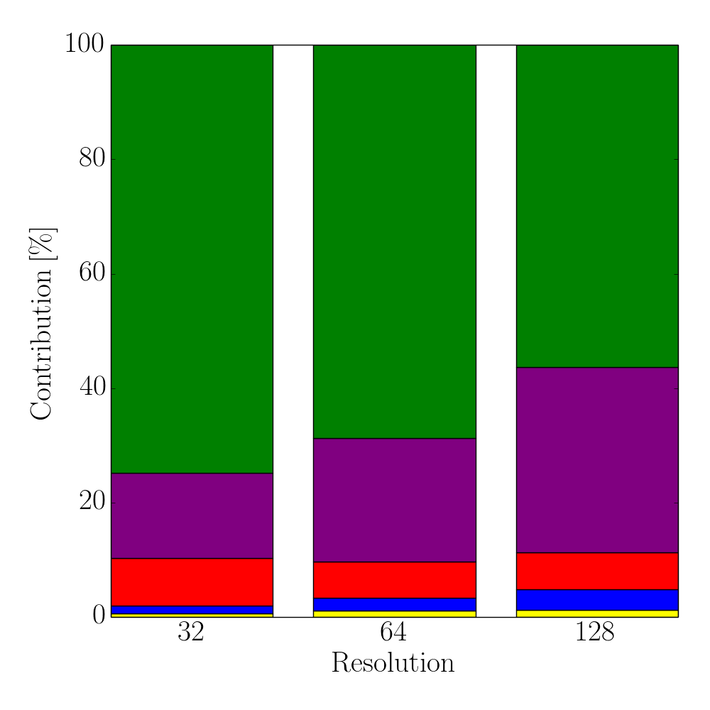
Figure 5.11: Contributions of the four major steps in the sparse flux calculation algorithm using one and 16 threads for different level-set resolutions: Initial partitioning of the cells for the sparse set (blue), initial flux calculation (red), iterative refinement (purple), and the corresponding flux calculation (green). Miscellaneous (yellow) accounts for any other occurring overhead within the sparse set algorithm, e.g., computing the local flux deviations from the global maximum flux.
5.6 Summary and Conclusion
A new iterative partitioning method for multi-material surface meshes for etching simulations, which play a key role in Process TCAD, was introduced in this chapter. It was shown that the flux calculation step for an etching simulation of a dielectric layer, as it occurs for example in the Dual-Damascene process, is significantly accelerated using the developed multi-material interface-aware approach. The method is based on the initial creation of a so-called sparse set which is subsequently refined with respect to a user-defined refinement condition. This condition is based on thresholds for the flux difference and the normal angle deviation between two adjacent points of the sparse set. Using different level-set resolutions for the underlying implicit surface representation, the obtained relative speedups with the new approach range from 1.9 to 7.0. As it is the case with almost every approximation method, the introduced novel multi-material interface-aware partitioning method introduces minor surface cell deviations between the dense and the sparse method, with the recorded maximal deviations being inside the vias. However, the deviations are below two surface mesh cells for the highest level-set resolution of 128, corresponding to about 0.6% of the via size. For the lowest level-set resolution of 32, the deviations stay below 0.7 surface mesh cells, i.e., 3% of the via size. To asses the strong scaling capabilities of the proposed method, a benchmark study using up to 16 threads was conducted. Almost linear scaling for both the dense and the sparse set method is achieved, using up to four threads. For higher thread counts the sparse set method experiences a kink in the recorded speedups, originating from the increased shares of the serial steps of the flux calculation process. Thus, the currently serially realized implementation of the iterative partitioning method limits the maximum speedup to roughly 50% of the theoretical limit. Nevertheless, the newly proposed sparse set multi-material interface-aware partitioning method is able to significantly outperform the conventional dense evaluation approach.