7.5 Explanation for Noise in TDDS Measurements
So far it has been shown that the eNMP model accounts for all features seen in the
time constant plots for the ‘normal’ as well as the ‘anomalous’ defects. Beyond that,
the model can also give an explanation for tRTN observed in TDDS (see
Section 1.3.4). The generated noise stems from defects switching forth and back
between states  and
and  . The associated charge transfer reactions
  do not
involve any intermediate states and are therefore simple NMP processes. It is
remarked here that the transitions
do not
involve any intermediate states and are therefore simple NMP processes. It is
remarked here that the transitions  require the energy minima
  and
and  in
the configuration coordinate diagram to be on approximately the same level at the
relaxation voltage. This is only the case for a group of defects whose energy minima
in
the configuration coordinate diagram to be on approximately the same level at the
relaxation voltage. This is only the case for a group of defects whose energy minima
 and
and  are energetically not far separated. In a TDDS measurement, the
investigated devices are stressed at a high
are energetically not far separated. In a TDDS measurement, the
investigated devices are stressed at a high  so that the defects are forced from the
state
so that the defects are forced from the
state  into the state
  or
or  . During this step, the defects undergo the
transition
. During this step, the defects undergo the
transition  into the state
  or even further into
  . The other
direct pathway
. The other
direct pathway  into the state
  or
or  is assumed to go over a large
barrier
is assumed to go over a large
barrier  . Therefore, the transition
  proceeds on much larger
timescales compared to
proceeds on much larger
timescales compared to  and can be neglected. After stressing, the
recovery traces are monitored at low
and can be neglected. After stressing, the
recovery traces are monitored at low  or
or  , respectively, at which the
energy minima of the states
, respectively, at which the
energy minima of the states  and
and  coincide and noise is produced.
However, the state
coincide and noise is produced.
However, the state  is thermodynamically preferred due to its energetically
lower position compared to the states
is thermodynamically preferred due to its energetically
lower position compared to the states  and
and  . When the defect returns
to its initial state
. When the defect returns
to its initial state  , the RTN signal disappears with a time constant of
 . The corresponding transition could be either
  or
or  with a time constant of
  or
or  , respectively (cf. Fig. 7.11). The
termination of the noise signal after a time period of
, respectively (cf. Fig. 7.11). The
termination of the noise signal after a time period of  is determined by the
minimum of these time constants. Consider that the NMP barriers
is determined by the
minimum of these time constants. Consider that the NMP barriers  and
and  must not be too large since otherwise trapping events will occur
too fast and are therefore not detected using a conventional measurement
equipment.
must not be too large since otherwise trapping events will occur
too fast and are therefore not detected using a conventional measurement
equipment.
Interestingly, there also exists a sort of defects which repeatedly produce noise for a
some time (see Section 1.3.4). This kind of noise has been referred to as aRTN
and will be discussed for hole traps in the following. Just as in the case of
tRTN, the noise signal is generated by charge transfer reactions between the
states  and
and  . The recurrent pauses of the noise signal (see Fig. 7.11)
originate from transitions into the metastable state
. The recurrent pauses of the noise signal (see Fig. 7.11)
originate from transitions into the metastable state  , which is electrically
indistinguishable from the state
, which is electrically
indistinguishable from the state  . These interruptions correspond to the time
during which the defect dwells in this state and no charge transfer reaction can
take place. Thereby it has been presumed that the NMP transition
. These interruptions correspond to the time
during which the defect dwells in this state and no charge transfer reaction can
take place. Thereby it has been presumed that the NMP transition  occurs on larger time scales than the return to the state
  through the
transition
through the
transition  . The slow capture time constant
  in Fig. 7.11 defines the
mean time interval during which noise is observed. Its value is given by
the inverse of the transition rate
in Fig. 7.11 defines the
mean time interval during which noise is observed. Its value is given by
the inverse of the transition rate  . The slow emission time constant
 corresponds to the mean time interval until the next noise period
starts.
corresponds to the mean time interval until the next noise period
starts.
One should keep in mind that defects showing an aRTN behavior can also be
responsible for tRTN seen in TDDS measurements. During TDDS stress, this sort of
defects are forced into one of the states  and
and  where they produce an RTN
signal. As in aRTN, they undergo a transition to the metastable state
where they produce an RTN
signal. As in aRTN, they undergo a transition to the metastable state  thereby
stopping to produce a noise signal. However, this special sort of defects is
characterized by a slow emission time constant
thereby
stopping to produce a noise signal. However, this special sort of defects is
characterized by a slow emission time constant  , which is much larger than the
typical measurement time of TDDS. As a consequence, the next transition back to
the state
, which is much larger than the
typical measurement time of TDDS. As a consequence, the next transition back to
the state  and the subsequent noise period are shifted out of the experimental time
window of TDDS and will not be recorded during the measurement run. According to
this explanation, tRTN can also be explained as a stimulated variant of
aRTN.
and the subsequent noise period are shifted out of the experimental time
window of TDDS and will not be recorded during the measurement run. According to
this explanation, tRTN can also be explained as a stimulated variant of
aRTN.
In summary, the eNMP can account for the features from the time constant plots and
is consistent with the observation of tRTN as well as aRTN. This fact is presented
here since it is regarded as an additional support for the validity of this
model.
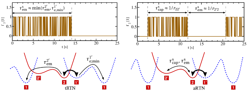
 the stress
voltage has been removed and the defect is in its positive state
the stress
voltage has been removed and the defect is in its positive state  . After a
time
. After a
time  the defect ceases to produce noise.
  and
and  related to the occurrence of noise.
The possibilities to escape from these states are shown by the thin arrows.
related to the occurrence of noise.
The possibilities to escape from these states are shown by the thin arrows.
 .
.