and
and  will be
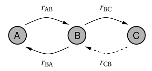
derived analytically in the following. The time constants observed in TDDS can be
calculated on the basis of first passage times of a two-step process (see Fig. 7.5).
will be
derived analytically in the following. The time constants observed in TDDS can be
calculated on the basis of first passage times of a two-step process (see Fig. 7.5).
In order to promote the understanding of the eNMP model, and will be
derived analytically in the following. The time constants observed in TDDS can be
calculated on the basis of first passage times of a two-step process (see Fig. 7.5).
 , provided that it was in the state
  but not in
state B at the beginning. In the eNMP model, one is only interested in the
transition times between the stable states
but not in
state B at the beginning. In the eNMP model, one is only interested in the
transition times between the stable states  and
and  , in which the defect dwells
most of the time. Since the metastable states
, in which the defect dwells
most of the time. Since the metastable states  and
and  are energetically
higher than their corresponding stable counterparts
are energetically
higher than their corresponding stable counterparts  and
and  , the defect
only remains temporarily in these metastable states. This is in agreement
with the condition for the first passage time that the system must not be
in state B at the beginning. As a result, the transition rates between the
states
, the defect
only remains temporarily in these metastable states. This is in agreement
with the condition for the first passage time that the system must not be
in state B at the beginning. As a result, the transition rates between the
states  and
and  can be reasonably described as the inverse of first passage
times.
can be reasonably described as the inverse of first passage
times.
 to
to
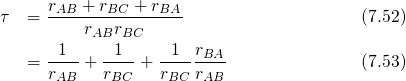
 . The first passage time of such a process is calculated by equation (7.52).
Consider that the transition rate
. The first passage time of such a process is calculated by equation (7.52).
Consider that the transition rate  , indicated by the dashed arrow, does
not enter this equation.
, indicated by the dashed arrow, does
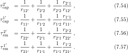
not enter this equation.The various transition pathways allowed in the eNMP model are summarized in the state diagrams of Fig. 7.6. The corresponding first passage times for the hole capture or emission read
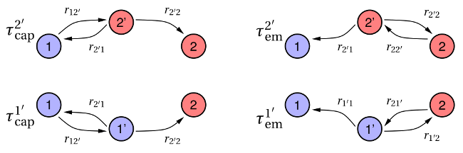
 and
and  . The superscript of
  denotes the intermediate
state, which has been passed through during a complete capture or the emission
event. Note that there exist two competing pathways for a hole capture event,
namely one over the intermediate state
denotes the intermediate
state, which has been passed through during a complete capture or the emission
event. Note that there exist two competing pathways for a hole capture event,
namely one over the intermediate state  and one over
  . Of course, the
same holds true for a hole emission event.
. Of course, the
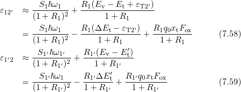
same holds true for a hole emission event.For studying the field dependence of these capture and emission times, the definition
( ) is used for
  and
and  in the expression for the NMP barriers (7.17):
Recall that the hole capture process can proceed from state  over one of the
metastable states
over one of the
metastable states  or
or  to the final state
  according to the state diagram of
Fig. 7.3. The corresponding capture time constants are denoted as
according to the state diagram of
Fig. 7.3. The corresponding capture time constants are denoted as  and
and  ,
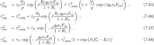
respectively, and will be discussed in the following. When the transition pathway
,
respectively, and will be discussed in the following. When the transition pathway
 is preferred, the capture time constant in the form of (7.52) is given by

 is
characterized by three distinct regimes, namely B, C, and D in Fig. 7.7.
is
characterized by three distinct regimes, namely B, C, and D in Fig. 7.7.
 is the dominant
rate meaning that the transition2
is the dominant
rate meaning that the transition2
 proceeds much faster than
  (cf. Fig. 7.8). Thus the pace
of the complete capture process (
(cf. Fig. 7.8). Thus the pace
of the complete capture process ( ) is determined by the second
transition
) is determined by the second
transition  , which is much slower and has a time constant of
  .
Since this second step is only thermally-activated,
.
Since this second step is only thermally-activated,  does not depend
on the oxide field. This is consistent with equation (7.65) at extremely high
negative oxide fields, at which both exponential terms become negligible
compared to
does not depend
on the oxide field. This is consistent with equation (7.65) at extremely high
negative oxide fields, at which both exponential terms become negligible
compared to  .
.
 approaches the
order of magnitude of
approaches the
order of magnitude of  and even falls below
  . Then the transition
 over the thermal barrier
  is undergone immediately after the
defect has changed from the state
is undergone immediately after the
defect has changed from the state  to
to  . Thus the kinetics of the
hole capture process are governed by the forward rate of the NMP process
. Thus the kinetics of the
hole capture process are governed by the forward rate of the NMP process
 . As a result,
  shows an exponential oxide field dependence,
which is reflected in the first term of equation (7.65). Note that the second
term is negligible due to its steeper exponential slope within this regime.
shows an exponential oxide field dependence,
which is reflected in the first term of equation (7.65). Note that the second
term is negligible due to its steeper exponential slope within this regime.
 is already outbalanced by
its reverse rate
is already outbalanced by
its reverse rate  (see Fig. 7.8) and the ratio of both rates determines
the oxide field dependence. This gives an increased exponential slope
originating from the second term of equation (7.65).
(see Fig. 7.8) and the ratio of both rates determines
the oxide field dependence. This gives an increased exponential slope
originating from the second term of equation (7.65).The transitions between these three regimes are smooth so that a curvature appears
in the time constant plots of  .
.
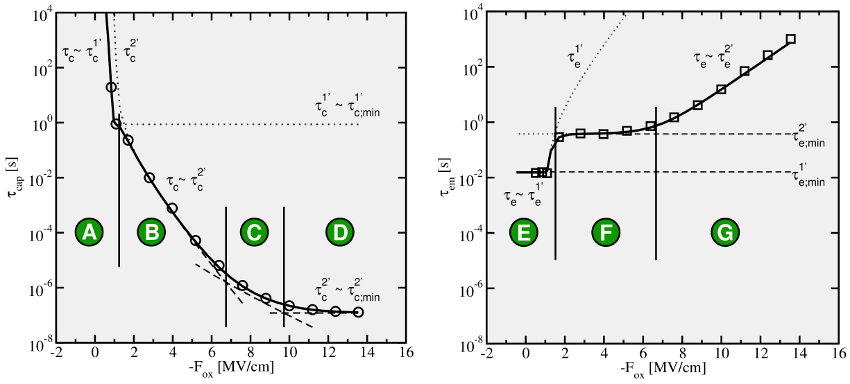
 (A, B, C, and D) are separated by
the thin vertical lines and labeled by the green circles with the capital letters.
The dotted curves
(A, B, C, and D) are separated by
the thin vertical lines and labeled by the green circles with the capital letters.
The dotted curves  show the capture processes over a metastable state
  .
The field dependence of
.
The field dependence of  within a certain regime is shown by the dashed
curve, which becomes constant if
within a certain regime is shown by the dashed
curve, which becomes constant if  is insensitive to
  . Right: The same
but for the hole emission time constants with the regimes (E, F, and G).
. Right: The same
but for the hole emission time constants with the regimes (E, F, and G).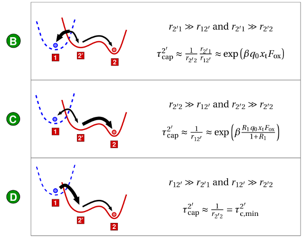
 . With higher oxide fields (B
  D) the blue potential (neutral
defect) is raised relative to the red one (positive defect). This is associated with
an increase of
D) the blue potential (neutral
defect) is raised relative to the red one (positive defect). This is associated with
an increase of  and a decrease of the reverse rate
  . In contrast to the
charge transfer reactions
. In contrast to the
charge transfer reactions  and
and  , the thermal transition
  is
not affected by the oxide field.
is
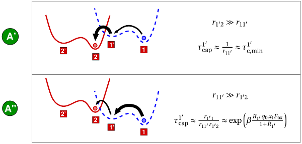
not affected by the oxide field.However, when the transition over the metastable state  is favored (regime A),
the capture time constant can be again formulated as a first passage time:
is favored (regime A),
the capture time constant can be again formulated as a first passage time:
 is situated above the state
  by definition,
 holds. Therefore, the expression (7.75) can be approximated by
which is characterized by only two regimes (A’ and A”) now.
holds. Therefore, the expression (7.75) can be approximated by
which is characterized by only two regimes (A’ and A”) now.
 is located relatively high
(see Fig. 7.9) and the transition rate
is located relatively high
(see Fig. 7.9) and the transition rate  exceeds
  . Therefore, the
first term of expression (7.76) vanishes and the field-insensitive transition
. Therefore, the
first term of expression (7.76) vanishes and the field-insensitive transition
 with a time constant of
  dominates
  .
.
 is shifted downwards in the
configuration coordinate diagram, thereby decreasing the transition rate
is shifted downwards in the
configuration coordinate diagram, thereby decreasing the transition rate
 . At a certain oxide field,
  falls below
  and the first term of
the expression (7.76) becomes dominant (regime A”). As a consequence,
and the first term of
the expression (7.76) becomes dominant (regime A”). As a consequence,
 governed by the field-dependent transition
  , which causes
the exponential term of the expression (7.66). Depending on the value of
, which causes
the exponential term of the expression (7.66). Depending on the value of
 , there exists a crossing point between the curves
  and
and  ,
marking the transition between the regime A and B. It is noted that the
NMP transitions in the regimes A, B, and C also involve a nearly negligible
,
marking the transition between the regime A and B. It is noted that the
NMP transitions in the regimes A, B, and C also involve a nearly negligible
 field dependence, which has already been present in the TSM for
instance.
field dependence, which has already been present in the TSM for
instance.The transition between A’ and A” yields a kink, which is visible in  of Fig. 7.7 (dotted line) but not in the overall hole capture time given by
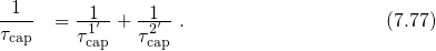
 .
.Also the hole emission process has the possibility to proceed over either the state  or
or  , with
  and
and  being the corresponding emission time constants (see
Fig. 7.10). For the transition pathway over
being the corresponding emission time constants (see
Fig. 7.10). For the transition pathway over  the emission time constant can be
expressed as:
the emission time constant can be
expressed as:

 applies,
  has only two regimes, labeled with the capital letters
F and G in Fig. 7.7.
has only two regimes, labeled with the capital letters
F and G in Fig. 7.7. 
 is shifted
upwards so that
is shifted
upwards so that  dominates and the field-dependent NMP transition
 determines the pace of
  . The sensitivity of
  to
the oxide field is reflected in the exponential term of equation (7.67).
to
the oxide field is reflected in the exponential term of equation (7.67).
 proceeds
much faster than
proceeds
much faster than  over the purely thermal barrier
  . Thus,
 is determined by the field-insensitive transition
  with a time
constant of
with a time
constant of  . It is important to note that the field independence
of this regime is experimentally observed in the time constant plots of
‘normal’ defects (cf. Fig. 7.4 left).
. It is important to note that the field independence
of this regime is experimentally observed in the time constant plots of
‘normal’ defects (cf. Fig. 7.4 left).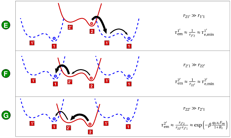
 .
.At a low oxide field (regime E), the state  is further shifted down, which
speeds up the NMP transition
is further shifted down, which
speeds up the NMP transition  and allows the pathway over the
metastable state
and allows the pathway over the
metastable state  . The corresponding emission time constant
  is given by

 the rate
  is negligible compared to
  and
and
 and the above equation simplifies to
 and
and  and is marginally disturbed by the rate
  . Then the states
  and
and  can be assumed to be in quasi-equilibrium.
 holds so that the trap occupancy
 is given by
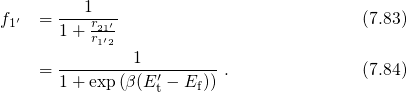
 is
equivalent to
is
equivalent to  . Furthermore, this equation can be used to simplify the
equation (7.68) as follows:
. Furthermore, this equation can be used to simplify the
equation (7.68) as follows: 
 falls below
  at a certain relaxation voltage, the state
  becomes occupied
and the emission time
becomes occupied
and the emission time  is determined by the field-independent transition
  with the time constant
  . By contrast, if
  is raised above
  , the state
  is underpopulated thereby slowing down the hole emission process. This occupancy
effect is reflected in the second term, which reacts sensitive to changes in
is underpopulated thereby slowing down the hole emission process. This occupancy
effect is reflected in the second term, which reacts sensitive to changes in
 .
.
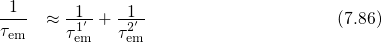
The overall hole emission time  follows from
 is shifted
below state
is shifted
below state  ,
,  reaches its minimum value and falls below
  . The resulting
drop in
. The resulting
drop in  is observed as the field dependence characterizing ‘anomalous’ defects
at weak oxide fields in TDDS experiments. As pointed out in Fig. 7.4, the
drop of
is observed as the field dependence characterizing ‘anomalous’ defects
at weak oxide fields in TDDS experiments. As pointed out in Fig. 7.4, the
drop of  occurs when the minimum of the state
  passes that of state
 , and is thus related to the exact shape of the configuration coordinate
diagram.
, and is thus related to the exact shape of the configuration coordinate
diagram.