Monte Carlo Methods require a large amount of uniformly distributed random numbers. In
computer simulations usually a sufficient long sequence of pseudo random numbers
is used, which makes the results reproducible and debugging of program code
generally easier.
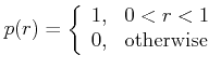
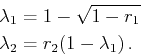
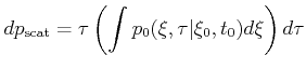
The probability density ![]() of a uniformly distributed random number
of a uniformly distributed random number ![]() is
is
 |
(4.1) |
 |
(4.2) |
| (4.3) |
| (4.4) |
 |
(4.5) |
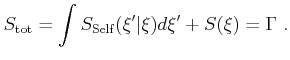
This method consists of two steps. It involves the probability density
![]() which is chosen so that it reproduces the original probability density
which is chosen so that it reproduces the original probability density
![]() as close as possible but with the constraint that a closed form of the
inverse distribution function can be found. In a first step a random number
as close as possible but with the constraint that a closed form of the
inverse distribution function can be found. In a first step a random number
![]() is generated with a probability density
is generated with a probability density
![]() with the condition
with the condition
| (4.6) |
During a Monte Carlo simulation the scattering rate depends in a complex way on
the carrier state. Therefore, calculating the time
![]() of the
next scattering event demands for high computing time. To speed up the
calculation of
of the
next scattering event demands for high computing time. To speed up the
calculation of
![]() the scattering rate can be rendered to a
constant upper bound value,
the scattering rate can be rendered to a
constant upper bound value, ![]() , by introducing an artificial scattering
process, the so called self-scattering [Jacoboni83] process. In the
following a scheme using piecewise constant
, by introducing an artificial scattering
process, the so called self-scattering [Jacoboni83] process. In the
following a scheme using piecewise constant ![]() -values is illustrated,
which is particularly suitable for FBMC.
-values is illustrated,
which is particularly suitable for FBMC.
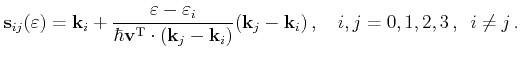
For the sake of a simplified notation the variables of a particle state are written as
| (4.8) |
 |
(4.9) |
Furthermore, the integral over the phase space volume and the summation over the band index is shortened as
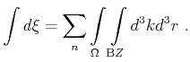 |
(4.10) |
 |
(4.11) |
 |
(4.12) |
 |
(4.14) |
| (4.17) |
 |
(4.18) |
| (4.22) |
| (4.24) |
 |
(4.25) |
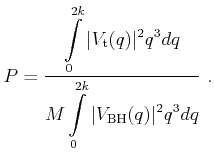
Instead of evaluating the ionized impurity scattering rate with the complicated
potential (3.48), a more efficient self-scattering scheme can be implemented
in a Monte Carlo simulator. Within this scheme the Brooks-Herring rate
multiplied by a factor ![]() is evaluated. Using (3.35) and (3.48)
is evaluated. Using (3.35) and (3.48) ![]() is chosen so that the following
relation is fulfilled for any
is chosen so that the following
relation is fulfilled for any ![]() in the interval
in the interval ![]()
| (4.26) |
A scattering rate of Brooks-Herring type is obtained which is always larger than the scattering rate resulting from the potential (3.48)
| (4.27) |
Here,
![]() is the scattering rate, which is evaluated with the
potential (3.48). Therefore a well defined probability
is the scattering rate, which is evaluated with the
potential (3.48). Therefore a well defined probability ![]() exists that a Coulomb
scattering event is accepted [Kosina97]
exists that a Coulomb
scattering event is accepted [Kosina97]
 |
(4.28) |
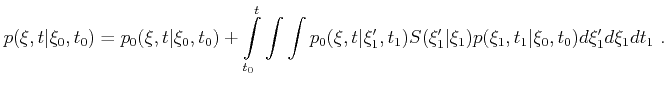
Instead of solving these integrals numerically a solution by means of Monte
Carlo integration can be found the following way. First a random number
![]() with the probability density
with the probability density
![]() is chosen. Then a second random number
is chosen. Then a second random number
![]() is chosen, which is evenly distributed between
is chosen, which is evenly distributed between
![]() . If
. If
![]() , the scattering event is accepted,
otherwise it is rejected and a self-scattering event is performed.
, the scattering event is accepted,
otherwise it is rejected and a self-scattering event is performed.
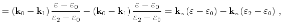
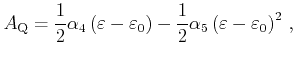
In this section, the basic layout of a rejection algorithm to select the final state of a carrier after a scattering event is shown.
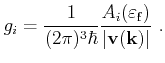
For scattering models with constant matrix elements‚
the scattering rates are proportional to the DOS at the carrier's final energy
![]() (see Section 3.3). Selection of a state after scattering
then relies mainly on the calculation of the contribution to the DOS of the
mesh elements including the particle's final energy. This is achieved by using
tetrahedral mesh elements and linear interpolation of the energy within the
mesh elements. The contribution
(see Section 3.3). Selection of a state after scattering
then relies mainly on the calculation of the contribution to the DOS of the
mesh elements including the particle's final energy. This is achieved by using
tetrahedral mesh elements and linear interpolation of the energy within the
mesh elements. The contribution ![]() to the DOS of the
to the DOS of the ![]() -th tetrahedron is
proportional to the intersection of the equi-energy surface
-th tetrahedron is
proportional to the intersection of the equi-energy surface
![]() [Lehmann72][Jungemann03]
[Lehmann72][Jungemann03]
The most time consuming task while computing a scattering event is the
selection of a final tetrahedron containing the final energy
![]() . Several tables are calculated once at start time of the
simulation to speed up this selection process.
. Several tables are calculated once at start time of the
simulation to speed up this selection process.
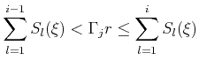
After a scattering process is selected the final energy
![]() of the
scattered particle is known and so the search for a final tetrahedron can be constricted to the tetrahedrons containing
of the
scattered particle is known and so the search for a final tetrahedron can be constricted to the tetrahedrons containing
![]() . Actually only tetrahedrons with a minimum energy in the range between
. Actually only tetrahedrons with a minimum energy in the range between
![]() and
and
![]() from the table of sorted tetrahedrons are
considered in this search.
from the table of sorted tetrahedrons are
considered in this search.
 |
(4.31) |
![\includegraphics[scale=1.4, clip]{figures/flow.ps}](img501.png)
|
The corresponding table indices
![]() and
and
![]() are calculated by a
binary search. Then a tetrahedron
are calculated by a
binary search. Then a tetrahedron ![]() is chosen randomly from this
interval. There is a small number of tetrahedrons in the considered interval
which do not contain
is chosen randomly from this
interval. There is a small number of tetrahedrons in the considered interval
which do not contain
![]() . These are sorted out within a first rejection
step.
. These are sorted out within a first rejection
step.
During a second rejection step the DOS within the tetrahedron has to be
evaluated using equation (4.29). Figure 4.1 shows a flow-chart of the selection procedure
with its two step rejection technique. Since the whole procedure is repeated
until the second rejection step is passed,
![]() has to be evaluated
frequently during the simulation.
has to be evaluated
frequently during the simulation.
After selecting the final tetrahedron ![]() ,
a final wave vector
,
a final wave vector
![]() has to be chosen within this
tetrahedron. Since equi-energy areas are planes and the group velocity is
constant within a tetrahedron, this problem is reduced to the determination of
a uniformly distributed random point on the equi-energy plane defined by
has to be chosen within this
tetrahedron. Since equi-energy areas are planes and the group velocity is
constant within a tetrahedron, this problem is reduced to the determination of
a uniformly distributed random point on the equi-energy plane defined by
![]() .
.
The equi-energy plane has the shape of either a triangle or a quadrangle as
depicted in Figure 4.9 and Figure 4.10, respectively. In the
case of a quadrangle, it is split into two triangles and one triangle is
randomly chosen according to the surface ratio. The final
![]() -vector is then determined with
-vector is then determined with
| (4.32) |
 |
(4.33) |
Within this work we mesh the first octant of the first Brillouin zone to represent the band structure of relaxed and biaxially strained Si (see Section 2.6). Because an octant is a larger volume than the irreducible wedge, this approach obviously increases memory consumption. However, it simplifies the manipulations needed when particles reach a boundary [Karlowatz07].
The energy bands are calculated for the irreducible wedge using the empirical pseudopotential method [Ungersboeck07a][Rieger93] and then transformed by coordinate permutation to completely fill the first octant. Two approaches of mesh generation employing structured and unstructured tetrahedral meshes are explored for several simulation setups.
The structured mesh is based on an octree approach. The domain to be meshed is devided into cubes and afterwards the cubes are divided into six tetrahedrons. To mesh the {111} surface of the Brillouin zone either one or five tetrahedrons have to be cut away from the six tetrahedrons forming one cube. The result is a structured tetrahedral mesh, whose surface is conform with the Brillouin zone boundary.
Figure 4.2(a) shows the
![]() -
-
![]() plane of the
first octant of the Brillouin zone with the contour plot of the energy of the
first conduction band. The main drawback of the octree approach is the
difficulty to implement a sufficiently flexible refinement strategy to
accomodate different mesh densities. In [Fischer99] an octree algorithm is
proposed which can deal with different mesh densities, but the refinement zone
is limited to a cubical region and is therefore not very flexible.
plane of the
first octant of the Brillouin zone with the contour plot of the energy of the
first conduction band. The main drawback of the octree approach is the
difficulty to implement a sufficiently flexible refinement strategy to
accomodate different mesh densities. In [Fischer99] an octree algorithm is
proposed which can deal with different mesh densities, but the refinement zone
is limited to a cubical region and is therefore not very flexible.
![\begin{figure*}\centering
\subfigure[Structured Mesh]
{\epsfig{figure =figures/...
... =figures/unstruct_iso_contour_2d_bw2.eps2,width=0.75\textwidth}}\end{figure*}](img514.png) |
A more flexible way of generating unstructured meshes is to use a mesh generator which can handle arbitrary point clouds with different point densities. In this particular work DELINK [Fleischmann99] was used to generate an initial, very coarse, unstructured mesh. For different energy bands this initial mesh was refined by the so-called tetrahedral bisection method. The basic idea of this method is to insert a new vertex on a particular edge, the refinement edge, of a tetrahedron, and to cut the tetrahedron into two pieces.
In literature one can find different improvements and specifications for this algorithm (see, for example [Arnold00]). One common problem is the detection of the refinement edge. In a mesh, tetrahedrons are not isolated and inserting a new vertex influences the whole refinement edge batch of the tetrahedron if the conformity of the mesh after the refinement step should be kept, which is normally the case. To guarantee good shaped elements, a recursive refinement mechanism was chosen. This approach produces very regular, almost isotropic elements.
To guarantee a conforming mesh during the refinement procedure, all tetrahedrons sharing a common refinement edge have to be divided. A tetrahedron is said to be compatibly divisible if its refinement edge is either the refinement edge of all other tetrahedrons sharing that edge or the edge is part of the boundary of the domain. If a tetrahedron is compatibly divisible, we divide the tetrahedron and all other tetrahdedrons sharing the refinement edge simultaneously. If a tetrahedron is not compatibly divisible, we ignore it temporarily and divide a neighbor tetrahedron by the same process first. This leads to the atomic algorithm [Kossaczký94]. Figure 4.3 illustrates the recursive refinement process, where one new vertex is inserted.
![\begin{figure*}\centering
\subfigure[Four tetrahedrons.]
{\epsfig{figure=figur...
...=figures/8_init_tets2.eps,width=0.36\textwidth}}
\vspace*{-0.3cm}\end{figure*}](img515.png) |
As an input to the mesher, regions of high point densities are pre-defined by
the known positions of the band-minima in the Brillouin zone of Si. The
dimension of this region is chosen such that the shifted band-minima of
strained Si are taken into account and so the same mesh is usable with
recalculated energy values for different amounts of strain. As every band has
its unique position of the band-minina, the meshes are calculated for each band
seperately. For the valence bands only one one mesh is used, which is refined
around the ![]() -point.
-point.
To demonstrate the benefits of mesh refinement four meshes are compared. A
fine one and a coarse one of each the structured and the
unstructured mesh type were generated. The number of points and tetrahedrons in the first
conduction band of these meshes are shown in Table ![[*]](crossref.png) .
.
Figure 4.4 shows the mean electron energy as a function of the electric field for bulk Si for both structured and unstructured tetrahedral meshes. As the curves for 300K and also for 77K are grouped very close together above 10kV/cm, it can be concluded that for practical purposes the accuracy of the results in the high field regime is about the same for all meshes. Figure 4.5 shows a similar result for the velocity as a function of the electric field. These results demonstrate that the unstructured meshes perform very well in the high energy regimes, despite they contain less mesh elements than the structured meshes in that areas.
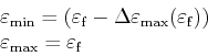
Figure 4.6 shows the normalized mean energy of electrons obtained
from FBMC simulation at thermal equilibrium. The result for the unstructured
meshes are in good agreement and converge for low temperatures to the
theoretical equilibrium value of
![]() . While the fine structured
mesh is sufficiently accurate at high temperatures, both structured meshes fail
completely at low temperatures. Figure 4.7 shows the low field
mobility of electrons. Again the coarse structured mesh fails, while fine
structured mesh is in fair agreement with the unstructured meshes.
. While the fine structured
mesh is sufficiently accurate at high temperatures, both structured meshes fail
completely at low temperatures. Figure 4.7 shows the low field
mobility of electrons. Again the coarse structured mesh fails, while fine
structured mesh is in fair agreement with the unstructured meshes.
Table gives an overview about computation times for
different meshes. The computation times are separated into the times for mesh
data structure build-up, which is required once at the beginning of the
simulation, and two typical velocity calculations, one in the low field regime
at ![]() kV/cm and a second one at
kV/cm and a second one at ![]() kV/cm. For every velocity calculated the
total amount of scattering events was set to
kV/cm. For every velocity calculated the
total amount of scattering events was set to
![]() . For the
calculations a computer system with a Intel
. For the
calculations a computer system with a Intel![]() Pentium
Pentium![]() 4 CPU with
4 CPU with ![]() GHz was used and the
user process CPU time was measured.
GHz was used and the
user process CPU time was measured.
One can clearly observe that the CPU time consumption is high for the structured meshes. This is mainly due the higher build-up times. With the much higher amount of mesh elements for the fine structured mesh, it takes a long time to compute the precalculated tables shown in the last section. The computation time using the unstructured fine mesh is approximately in the same range as for the coarse structured mesh, but one has to keep in mind, that the structured mesh fails completely for the average kinetic energy at temperatures less than room temperature, where the coarse unstructured mesh still gives reasonable results (see Figure 4.6).
In conclusion, the tetrahedral meshes offer a very good potential for refinement techniques. Simulation results in the high field regime show similar accuracy for properly refined meshes as for structured octree-based meshes with more than ten times the amount of tetrahedral elements. Simulations of electron mobility and mean electron energy in the low field regime show much better accuracy for refined meshes than octree-based meshes, particularly for simulations at low lattice temperatures.
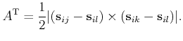
As shown in the last section the contribution of the tetrahedrons at a certain
energy to the DOS has to be evaluated very frequently during a FBMC
simulation. Therefore it is important to implement a CPU time efficient
calculation algorithm. According to
(4.30) the crucial step for the calculation of the DOS is to obtain the areas
![]() of the intersecting equi-energy planes of all contributing tetrahedrons
of the intersecting equi-energy planes of all contributing tetrahedrons
![]() .
.
In a first step the table of sorted tetrahedrons as defined in the last section is used to efficiently find tetrahedrons which intersect the considered energy surface. In the following both a conventional way to obtain this area and a more efficient approach based on the use of pre-calculated coefficients are presented. For the conventional calculation of the equi-energy plane the intersection points of the plane with the tetrahedron's edges are determined first.
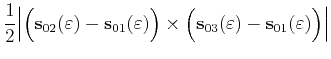
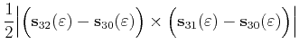
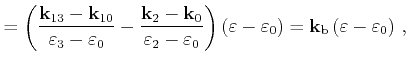
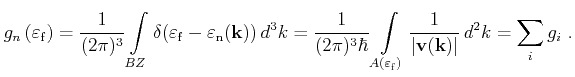
With the vectors ![]() to
to ![]() of the tetrahedron's
corners as depicted in Figure 4.8 the edges are derived as
of the tetrahedron's
corners as depicted in Figure 4.8 the edges are derived as
| (4.34) | |||
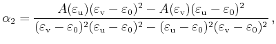
To save computation time the calculation of intersection planes can be
optimized by introducing area coefficients [Jungemann03], which are calculated
in a pre-processing step and stored for each tetrahedron. The tetrahedron's
vertices
![]() , and
, and
![]() carry the energies
carry the energies
![]() ,
,
![]() ,
,
![]() , and
, and
![]() .
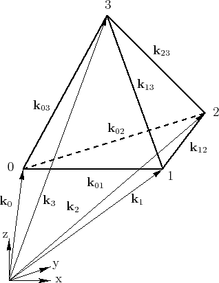
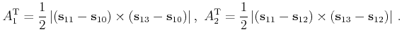
The energy
.
The energy
![]() changes linearly along the edges and is proportional to the
parameter
changes linearly along the edges and is proportional to the
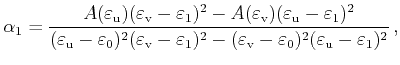
parameter ![]() (4.37). Therefore for the case of a triangular shaped
slice as shown in Figure 4.9 we obtain for the area
(4.37). Therefore for the case of a triangular shaped
slice as shown in Figure 4.9 we obtain for the area
![]()
| (4.40) |
 |
(4.41) | ||
 |
(4.42) | ||
 |
(4.44) |
 |
(4.45) |
 |
(4.46) |
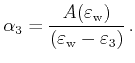
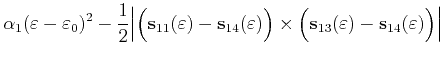
For the special case
![]() , an area calculation
with equation (4.44) fails because both triangle areas become
infinite. In this case another parameterization with the parameters
, an area calculation
with equation (4.44) fails because both triangle areas become
infinite. In this case another parameterization with the parameters ![]() and
and
![]() can be used, which is derived in the following.
First the quadrangle shaped intersection area is split into two triangles with areas
can be used, which is derived in the following.
First the quadrangle shaped intersection area is split into two triangles with areas
![]() and
and
![]()
 |
(4.48) |
 |
 |
(4.49) |
 |
 |
(4.50) |
 |
 |
(4.51) |
 |
Now, the area
![]() of the quadrangle can be written in
a parameterized formulation
of the quadrangle can be written in
a parameterized formulation
 |
(4.52) |
| (4.53) |
| (4.54) |
As shown in Section 4.5 it is convenient to use tetrahedral meshes for discretization of the Brillouin zone. It has also been shown that frequently used values like the area coefficients can be precalculated to improve performance during simulation. These values are stored related to the tetrahedral mesh elements, where they are either connected to the vertices, the surfaces or the volume.
The numbering of the vertices of each tetrahedron is sorted after increasing energies as explained in Section 4.4. The energies und positions of the vertices are stored in a table.
There are also several precalculated values with are connected to the
tetrahedron volumes: the energy gradient, which is used to calculate the group
velocity, the area-coefficients ![]() to
to ![]() (see
Section 4.6), and the upper bounds for the scattering rates for
different types of scattering mechanisms.
(see
Section 4.6), and the upper bounds for the scattering rates for
different types of scattering mechanisms.
For each of the four surfaces of a tetrahedron the type of the surface and a pointer to the neighbor tetrahedron are stored. Figure 4.11 shows the definition of the surface types. This value is used for efficient detection of the surface that would be crossed when a carrier has reached a border of the meshed part of the Brillouin zone. If the surface of the tetrahedron is inside of the meshed domain then the value of the surface type is defined as zero.
![\includegraphics[width=0.6\linewidth]{figures/surface7_3.eps}](img618.png)
|
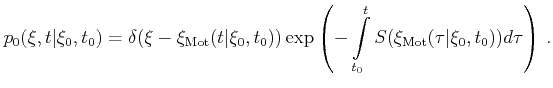
The Boltzmann equation can be solved either
with a given
electric field or with a selfconsistent field using an iteration scheme as
shown in Figure 4.13. After each time step ![]() the carrier
concentration is evaluated and the Poisson equation is solved
the carrier
concentration is evaluated and the Poisson equation is solved
for the electrostatic potential ![]() which in turn gives a new field for the
next iteration step. In (4.55)
which in turn gives a new field for the
next iteration step. In (4.55) ![]() denotes the dielectric constant
and
denotes the dielectric constant
and ![]() is the space charge density
is the space charge density
| (4.56) |
![\includegraphics[scale=1.01, clip]{inkscape_fig/MC-flow3.eps}](img624.png)
|
![\includegraphics[width=0.63\linewidth, clip]{figures/HighEnSispad.eps}](img516.png)
![\includegraphics[width=0.63\linewidth, clip]{figures/HiVelSispad.eps}](img517.png)
![\includegraphics[width=0.63\linewidth, clip]{figures/emean4.eps}](img518.png)
![\includegraphics[width=0.64\linewidth, clip]{figures/zfldMob4.eps}](img519.png)
![\includegraphics[width=0.6\linewidth]{figures/areacoefftri4.eps}](img565.png)
![\includegraphics[width=0.6\linewidth]{figures/areacoeffquad2.eps}](img596.png)
![\includegraphics[width=0.6\linewidth]{figures/neighbortypes.eps}](img617.png)