Lagrangian Formalism

5.2 Lagrangian Formalism

As Newton’s ideas and methods were adopted and applied to address problems of increasing sophistication its limits were also made apparent by the increase in the complexity of the used notation. Consequently, further development had the goal of addressing these shortcomings by simplifying calculations and establishing the foundations for a wider variety of treatable problems. Therefore, computational methods and notations to handle the increasing intricacies of the posed problems have been developed by Euler [64], Laplace [85] and Lagrange [86], without altering the fundamentals or the nature of Newton’s world. Where Newton’s description focuses on forces and accelerations using second order diﬀerential equations, the Lagrangian formulation recasts them as a set of ﬁrst order diﬀerential equations. It does so by redirecting attention from the explicit treatment of forces and accelerations to expressions linked to energy. Starting from an expression for Newton’s second law

dp- = f, (5.8) dt

the term for the force term may be decomposed into a part which can be represented using a potential and a remaining part.

dp ∂ --- = − ---V + ˆf (5.9) dt ∂r

Furthermore, the momentum $p$ is linkable to kinetic energy $T$ and expressible as

d p = d˙rT (˙r). (5.10)

Inserting into (5.9) yields

( ) -d- -d- ∂-- ˆ dt d˙r T(˙r) + ∂rV = f. (5.11)

The two terms of energy in this formulation are collected into a single expression as the diﬀerence of kinetic and potential energy

L = T − V (5.12)

called the Lagrangian. As such this Lagrangian contains components from the base manifold (Deﬁnition 37) as well as the tangent spaces (Deﬁnition 48) and is thus a mapping.

L : 𝒯 ℳ → ℝ (5.13)

Based on the Lagrangian, a motion takes the form

( ) d ∂ ∂ --- --L − ---L = ˆf, (5 .14) dt ∂˙r ∂r

which is called the Euler-Lagrange equation. While the Euler-Lagrange equation may seem to add to the overall complexity, the step to describe the evolution of a system using the scalar quantities of energy results in an overall simpliﬁcation as this notation remains invariant to a larger group of transformations and it becomes easier to apply constraints. The conﬁguration space is now generalized to a manifold, so that the coordinates which previously described a location in the physical world are now extended to abstract degrees of freedom. These abstracted degrees of freedom are no longer required to have physical dimensions such as position or velocity, but may in fact be dimensionless. Regardless of the physical dimension associated to the degrees of freedom, they are speciﬁed given as $q$ and $˙q$ , where $q$ corresponds to a base manifold $𝔐$ , $˙q$ is from the tangent space $TM.$ Thus this description can be summarized to take place in the tangent bundle $TM$ . Where previously a location, a velocity and an acceleration were required, it is now suﬃcient to provide a point in this tangent bundle, called the conﬁguration space. This does not change the Galilean structure of the world, however.

A trajectory which is used to describe a motion within the manifold $𝔐$ (Deﬁnition 35) may be associated with a curve (Deﬁnition 45) in the tangent bundle $T M$ (Deﬁnition 52) of $𝔐$ using a lift (Deﬁnition 26). Among all of the possible choices to lift a curve $γ$ , the one of the form

γ ∈ 𝔐 → (γ, ˙γ) = ¯γ ∈ TM , (5 .15)

which associates at every point the curve passes through its tangent vector, is called a natural lift.

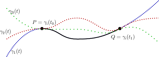
The curve to be lifted connects a starting point to an end point, thus changing the description from an initial value problem, to a boundary value problem. In order to appreciate the geometric nature of Lagrange’s formalism a short exploration of the concepts behind the distance of two points in a more traditional geometric setting is explored.

Using the clearly geometric construction presented in Section 4.8, with the Lagrangian $L$ taking the place of the metric ﬁeld, it is possible to evaluate the Lagrangian along a lifted curve and, again using the notion of a curve integral (Deﬁnition 95), assign values, called actions, to sections of any curve in the following fashion

∫ ∫ ∫ S = [t,t]L (¯γ (t),t)dt = [t,t]L(γ, ˙γ,t)dt = [t ,t]L (q, ˙q,t)dt, (5 .16) 0 1 0 1 0 1

where the parameters $t0$ and $t1$ correspond to the points $P$ and $Q$ as indicated in Figure 5.2. In mimicking the deﬁnition of distance, this allows to distinguish the various trajectories from each other, thus providing a selection criterion in the form of the extrema which can be derived using a simple homotopy (Deﬁnition 32) for variation, as can be shown in a short calculation.

d ∫ S = --|s=0 L(γ + sη, ˙γ + s˙η)dt = 0 (5.17) ds [t0,t1]

Setting

α = γ + sη, (5 .18)

it follows

∫ ∫ [ ] S=d| L(α,α˙)dt = -∂-L(γ, ˙γ)∂γ-+ ∂--L(γ,γ˙)∂˙γ- dt = 0. (5.19) dss=0 [t0,t1] [t0,t1] ∂γ ∂t ∂˙γ ∂t

Upon shortly examining the last term in this expression, it is found that

∫ ∂ ∂˙γ ∫ ∂ ( ∂ ) ∂γ ---L(γ,γ˙)---dt = − --- --L (γ, ˙γ) --dt, (5 .20) [t0,t1]∂γ˙ ∂t [t0,t1]∂t ∂˙γ ∂t

which, when applied, ﬁnally results in the expressions

∫ [ ( ) ] ∂ ∂ ∂ ∂t- ∂γ˙L(γ, ˙γ) − ∂-γL (γ, ˙γ) ˙γdt = 0, (5 .21) [t0,t1]

which can only hold in general, if the integrand itself vanishes. This condition is found to be equivalent to the Euler-Lagrange Equation 5.14. This means that from all possible curves $γi$ , which pass through the given points $P$ and $Q$ , as shown in Figure 5.2, the actual realization can be found by the minimization of the action deﬁned in Equation 5.16 as in this case the equations of motion in the form of the Euler-Lagrange Equation are met.

Figure 5.2: Lagrangian evaluated on sections of curves connecting the points $P$ and $Q$ .