| | |
Where previous comments regarding implementations dealt with classical settings, the following will touch upon the subject of the intangible world of quantum mechanics, which was ever so briefly discussed in Section 5.7. In contrast to the classical description the quantum world allows non-local coherent phenomena. The influence of these effects usually diminishes, when going beyond small scales of time and space, until finally, the macroscopic world appears in its classical beauty.
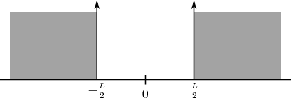
The setting of quantum mechanics shall serve as an example of the application of the presented abstractions of implementation. The case of the simple infinite square quantum well, illustrated in Figure 7.2, is well suited to provide an expressive example. Using Schr¨odinger’s equation (Equation 5.63) the solution to the infinite square well is found to read

Subjecting this analytic expression to the Wigner transformation given in Equation 5.71, again yields an
analytic expression for the Wigner function  defined on the phase space, which takes the
shape
defined on the phase space, which takes the
shape
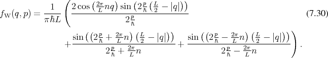
 , but also on a momentum
  as is consistent with the outlines provided in Section 5.7 and originally
in Section 5.3. This expression can easily be evaluated in a point wise manner, to yield
a scalar field (Definition 61) defined on the phase space. The evaluation in the discrete
setting of the digital computer proceeds by iterating over all points, which represent the
phase space and evaluating an expression encapsulating the prescription corresponding to
Equation 7.30.
as is consistent with the outlines provided in Section 5.7 and originally
in Section 5.3. This expression can easily be evaluated in a point wise manner, to yield
a scalar field (Definition 61) defined on the phase space. The evaluation in the discrete
setting of the digital computer proceeds by iterating over all points, which represent the
phase space and evaluating an expression encapsulating the prescription corresponding to
Equation 7.30.
This procedure is illustrated in the following snippet of code which uses the traversal capabilities provided by the GSSE as well as functional mechanisms in the spirit of Boost Phoenix [34]. It should be noted that the described procedure is fit to be used with structured grids as well as unstructured meshes, since topology based traversal is handled by the GSSE. Furthermore, it is also important to note that the traversal of the phase space nodes is completely independent of the dimension of the phase space. The functional expression used to compute the value of the scalar field needs to be able to deal with the dimensionality it is provided with. In this particular case the analytical prescription to obtain the phase space description corresponding to a particle in the infinite square quantum well can be extended to, in theory, arbitrary dimensions, albeit visualization of the resulting phase spaces is no longer easily possible.
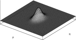
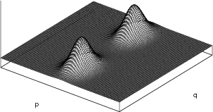
The results obtained in this fashion are illustrated in Figure 7.3 and Figure 7.4 for different values of
 , corresponding to different Eigenstates.
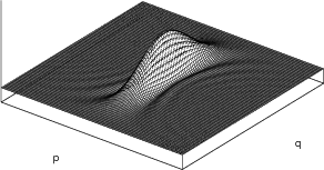
 ) in an
infinite square quantum well.
) in an
infinite square quantum well.
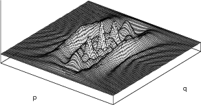
 ) in
an infinite square quantum well.
) in
an infinite square quantum well.
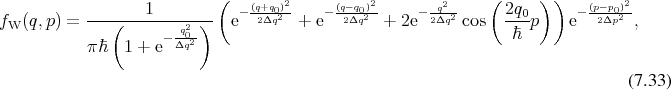
The bound states of a contained particle already are profound expression of quantum behaviour. Quantum mechanics using wave functions, however, allows for additional effects. The following example shall illustrate that such effects also find their expression, when using the phase space description. To this end a particle which is represented by a wave packet of the following form
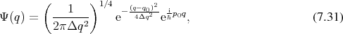
where  and
and  are the central position and the mean momentum respectively and
  represents
the width of the wave packet, shall be considered. Subjecting Equation 7.31 to the Wigner
transform (Equation 5.71) readily yields the phase space representation which can be given
analytically as
represents
the width of the wave packet, shall be considered. Subjecting Equation 7.31 to the Wigner
transform (Equation 5.71) readily yields the phase space representation which can be given
analytically as

Again using the traversal capabilities of the GSSE, the evaluation of this expression on the phase space
is identical to the previous case with the exception of supplying an appropriate functor in
accordance with Equation 7.32. Figure 7.5 provides an illustration of this wave packet in
phase space, thus depending on both location  and momentum
  , centred at the origin.
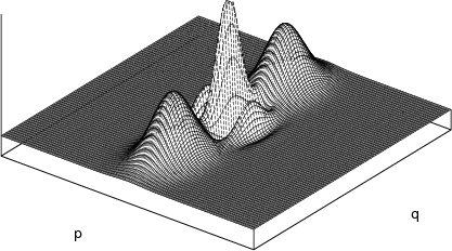
Moving beyond a single particle and thus a single wave packet, two particles in proximity to one another are considered. Proceeding by simply adding the two pseudo density functions resulting from the wave packets, a result as in Figure 7.6 is obtained, which corresponds to classical expectations regarding the interactions of particles.
The quantum mechanical setting, however, also allows for a different case, which can be explored by adding the wave functions comprising the two individual wave packets before applying the transformation to phase space. Proceeding in this manner yields the expression
| | |