Bordering Two Worlds Again

7.4 Bordering Two Worlds Again

While both of the extremes, the quantum setting as well as the classical world in their pure forms are well covered by powerful descriptions with respect to both, theory as well as application, the realm between them remains problematic, since both descriptions are driven to extremes of their validity.

In an attempt to bridge the gap between the two worlds in the setting of solid state physics, the following scheme has been developed which calculates an estimate for the modiﬁcation of a coherent solution as obtained by quantum mechanics, under the inﬂuence of classical scattering.

The following primarily uses the wave vector $k$ instead of the momentum $p$ in the descriptions, as is customary in solid state physics. Furthermore, it may be beneﬁcial to forgo the use of the full structure as presented in Equation 5.75 in Section 5.7 and decompose the description in the following manner

( ) ∫ ∂-+ ℏkx-∂-- fw(x,k) − Vw(x,kx ′ − kx)fw(x, k′,kyz)dkx′ = 0, (7 .34) ∂t m ∂x x

where $Vw$ is called the Wigner potential [99][135]. This is the basis for further simpliﬁcation. Under the assumption that $Vw$ locally varies at most linearly, a classical limit for this expression can be recovered [136] in the form

∫ V (x,k ′ − k )f (x,k′,k )dk ′ = − q-E-∂-f (x, k ,k ), (7 .35) w x x w x yz x ℏ ∂kx w x yz

where $q$ is the charge and $E$ the electric ﬁeld. Furthermore, the considerations are given here for one spatial dimension. The remaining two dimensions are assumed to be in equilibrium thus imposing a form for the coherent Wigner function $fcw$ of

2 ℏ2(k′+k′) f c(x,k) = fc(x, k )--ℏ----e− --2mykT-z- (7.36) w w x 2πmkT

using Maxwell-Boltzmann statistics, reminiscent of the Equilibrium provided in Equation 7.1. The same procedure is applicable to more than one dimensions, the requirement of a quantum mechanical solution, which is not easily available due to excessive numerical costs of computing a full density matrix required as input, make it diﬃcult in reality.

7.4.1 Wigner Boltzmann Equation

The Wigner Boltzmann equation [137] is obtained by combining elements of Equation 7.34 describing coherent transport and Boltzmann’s equation, as given in Equation 5.38 which includes scattering. The combination of the scattering operator and the coherent quantum expression in one dimension can be given as

∫ -∂- ′ ′ ′ ξ∂x fw(x,k ) = Vw(x, kx − kx)fw(x,kx,kyz)dk x+ (7.37) ∫ S(k ′,k )fwdk ′x − λ(k )fw (x,k),

where $k$ is speciﬁcally decomposed into the components $kx$ and $kyz$ .

The deviation $Δ fw$ of the true Wigner distribution $fw$ from the purely coherent $c fw$ is expressed as

f Δ(x,k ) = fw(x,k ) − f c(x, kx). (7.38) w w

This correction to the coherent case then satisﬁes the following equation

∂ ∫ ξ---fΔw (x, k) = Vw (x,k ′ − k)fwΔ(x,k ′)dk ′ (7.39) ∂x ∫ ′ Δ ′ ′ Δ + S (k ,k)fw (x,k )dk − λ(k)fw (x,k) ∫ + S (k′,k)fcw(x, k′)dk ′ − λ (k )fcw(x,k ),

which is treatable in the same fashion as Boltzmann’s equation in Section 5.6 to obtain an integral representation. To this end the equation is rewritten to read

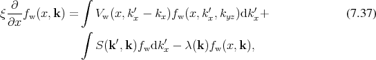
[ ∂ ] ∫ ξ--- + λ(k) fΔw (x, k) = Vw (x,k ′ − k)fwΔ(x,k ′)dk ′ (7 .40) ∂x ∫ ′ Δ ′ ′ + S (k ,k)fw (x,k )dk ∫ + S (k′,k)fc(x, k′)dk ′ − λ (k )fc(x,k ), w w

which again admits an integrating factor of the form $− ∫ λ(τ)dτ e$ . Thus the integral form of the correction equation becomes

[ ∫0 ]0 ∫ ∫ ∫0 fΔw(x,k)e− t λ(τ)dτ = Vw (x,k′ − k)fΔw (x, k′)dk′e− t λ(τ)dτdt (7.41) tb ∫[tb,0]∫ ′ Δ ′ ′− ∫0λ(τ)dτ + S (k ,k )fw (x, k)dk e t dt ∫[tb,0]∫ ′ c ′ ′− ∫t0λ(τ)dτ + S (k ,k )fw(x,k )dk e dt ∫[tb,0] ∫ − λ (k)fc(x,k )e− 0t λ(τ)dτdt. [tb,0] w

A further reduction can be applied to this expression by using the assumption that the zeroth order of correction already provides a reasonably good approximation. This assumption shall be checked with the implementation, given in Figure 7.11. Thus, foregoing the terms including $fwΔ$ on the right hand side, which corresponds to keeping only the zeroth order term, the expression reduces to contain only terms including $f c w$ which is assumed to be known from coherent calculations.

∫ ∫ fΔw (x, k) = S(k′,k)fcw(x, k′)dk ′e−λ(k)(−t)dt (7.42) [tb,0] ∫ c −λ(k)(−t) − λ(k)fw (x,k)e dt [tb,0]

The restriction to one dimension of this expression is obtained by integrating over $kyz$ , thus giving

∫ ∫ ∫ Δ ′ c ′ ′−λ(k)(−t) fw (x,kx) = S (k,k )fw(x,k )dk e dkyzdt (7.43) ∫[tb,0]∫ c −λ(k)(−t) − [t ,0] λ(k)fw(x,k )e dkyzdt. b

Inverting the passage of the parameter in the trajectories, results in a description of the form

∫ ∫ ∫ fΔw (x,kx) = S (k ′,k )fcw(x − vxt,k′)dk′e−λ(k)tdkyzdt (7.44) ∫[0,|tb|]∫ c − λ(k)t − λ (k)fw(x − vxt,k)e dkyzdt, [0,|tb|]

which will be used for further derivations from this point forward. Additionally $tb$ will be set to correspond to a positive value of the parameter without further particular indication thereof.

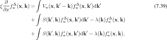
Rearranging and enhancing the last expression to extract representations identiﬁable as probabilities as was done for the derivations following Equation 7.10 gives

∫ ∫ ∫ { S(k ′,k )} { } fΔw(x,kx) = -------- λ(k )e− λ(k)t fwc(x − vxt,k′)dk ′dkyzdt (7.45) ∫ [0,tb]∫ ¯λ (k ′) { −λ(k)t} c − λ(k)e fw(x − vxt,k)dkyzdt, [0,tb]

which again employs the same basic components recognizable as probabilities as in Section 7.2. Thus although the algorithm is diﬀerent, the components for trajectories (Deﬁnition 45) and scattering mechanisms, which ﬁtted the backward Monte Carlo algorithm can again be used for calculations. Each of the integrals is evaluated separately. The Monte Carlo procedure for the ﬁrst integral is summarized as follows:

Initialize an electron state at a selected point of the discretized simulation domain.
Evaluate the scattering expression for the chosen state.
Follow the trajectory initialized from the after scattering state to the next scattering event.
Add the value of $fc w$ to an estimator corresponding to the point at the end of the trajectory.

The second integral term lacks the expression for the scattering probability, thus the algorithm can be given as:

Initialize an electron state at a selected point of the discretized simulation domain.
Follow the trajectory initialized from the after scattering state to the next scattering event.
Add the value of $fcw$ to an estimator corresponding to the point at the end of the trajectory.

The procedures for both integrals are performed using a subdivision of phase space into a structured grid, which deﬁnes the topology, as discussed in Section 6.3, and an estimator is associated with every grid node. This grid is then traversed and the two outlined algorithms are applied starting at every grid node, thus sampling phase space. The initialization of the electron states at every point has to take into account the decomposition into $k x$ and $k yz$ components. Therefore, the $yz$ components are initialized assuming equilibrium, while the $x$ component is initialized corresponding to the phase space position indicated by the grid. The grid is also used to hold parameters for the trajectories, thus making local modelling available, as described in Section 6.5. The local scattering mechanisms can reuse the know how of already existing codes, either directly, by extending the old code base, or by applying the methodology described in Section 7.2.3 to facilitate incorporation into a new frame work.

7.4.2 Approximation to Quantum Eﬀects in Semiconductor Devices

The derived correction is applied to a resonant tunnelling diode (RTD), as it combines quantum mechanical features with classical inﬂuence due to scattering. The resonant eﬀect is clearly due to quantum phenomena, yet the dimensions of the device may be such that scattering will disturb any purely coherent solution.

The structure of the device is given Figure 7.8, where the quantum well at the centre of the device is $4nm$ wide. The barriers have a thickness of $1nm$ and a height of $3eV$ . The active device is surrounded by several microns of contact region on both sides, where the distribution of charge carriers is undisturbed by the operation or structure of the device. This apparently inert region of the device has proved itself to be very important for the accuracy of the calculations due to the presented algorithm as is demonstrated in the later Figure 7.13.

Figure 7.8: Potential proﬁle of the simulated RTD. The $4nm$ wide quantum well is surrounded by $1nm$ barriers with a height of $0.3eV$ , applied is $0.3V$ bias.

The derivations critically depend on data corresponding to the coherent quantum case represented by $fcw$ . As outlined in Section 5.7 it can be obtained from a density matrix representation by means of transform as shown in Equation 5.71. This density matrix can be eﬃciently provided using a Non-Equilibrium Green’s Function (NEGF) [138][139][140] procedure. After the input has been subjected to the transformation, thus resulting coherent Wigner function representation serves as direct input for the Monte Carlo algorithm. An example of the Wigner representation corresponding to an RTD device is depicted in Figure 7.9.

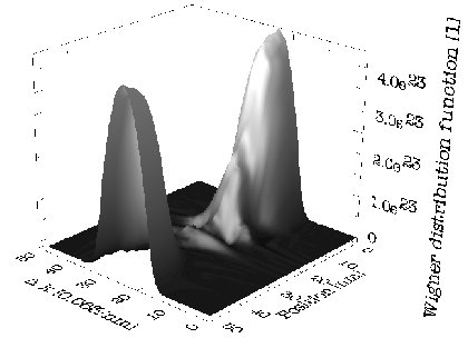
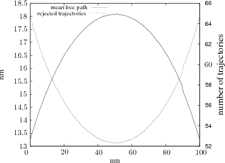
Figure 7.9: The coherent Wigner function $fwc$ obtained from transforming the coherent density matrix provided by a NEGF procedure.

The stochastic nature of the Monte Carlo approach makes veriﬁcation and debugging of implementations tedious. Therefore, simple test cases are of great importance to quickly detect and eliminate anomalies. One such possibility presents itself, when recording the length of trajectories, since every point is used to generate a trajectory which is either absorbed at the boundary or terminated by a scattering event, it is expected that trajectories will be shorter in the boundary regions. An investigation using histograms, shows that this is indeed the case as shown in Figure 7.10.

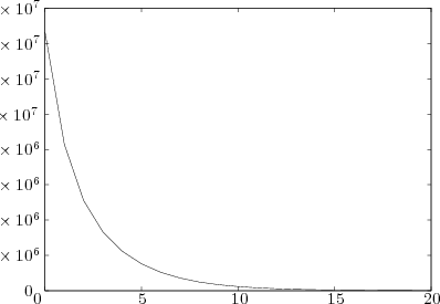
Figure 7.10: Histogram of the trajectories which leave the device and mean free path for trajectories which end in the device.

Furthermore, the assumption that the correction is mainly inﬂuenced by the ﬁrst scattering event can be gauged, by continuing the evolution past the ﬁrst collision and continuing the trajectory, until it reaches a boundary.

Figure 7.11: Number of trajectories still within the device versus the number of scattering events.

Figure 7.11 shows a steep decline in the number of trajectories still continuing within the domain of interest as the number of scattering events increases, corresponding to approximately an order of magnitude per scattering event.

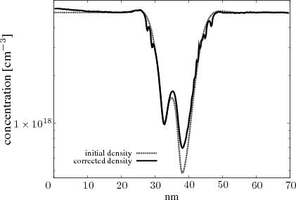
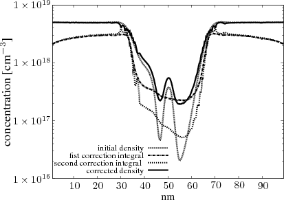
Finally, having established a means to estimate the validity of the assumption of considering only the ﬁrst order terms the procedure can be applied and the results are presented in Figure 7.12.

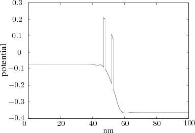
Figure 7.12: Density distribution in the device under $0.3V$ bias, presented in logarithmic scale.

The initial concentration, as obtained calculated from the density matrix is adapted by the scattering, increasing the concentration in the quantum well. It should be pointed out, however that this calculation is not self consistent that is the electric ﬁeld is kept constant throughout the simulation and not updated due to the shift of charge carriers. The procedure can be reﬁned to include such updates, by using the newly obtained distribution to calculate a new electric ﬁeld and also calculating a new density matrix. This new data can then be reapplied to the same procedure. The importance of adhering to the assumptions used in the theoretical derivations of the Monte Carlo procedure is illustrated in Figure 7.13.

Figure 7.13: An RTD with too short contact regions results in erroneous results at the contacts.

The derivation assumes that the contact regions are in equilibrium, which is not met precisely in the input for the calculation depicted in Figure 7.13. The discrepancy is not visible directly in the given ﬁgure, as there is seemingly no disturbance due to the ﬂatness of the contacts. However, applying the derived algorithm reveals that curiously the correction increases in the left contact, which by initial assumption should remain its ﬂat equilibrium conﬁguration. Examining the boundary conditions, revealed a deviation from equilibrium. When correcting this irregularity by extending the bounding contact regions, the results shown in Figure 7.12 are obtained.