

4 Level-Set Method for Anisotropic Wet Etching and Selective Epitaxy
During semiconductor fabrication processes, the semiconductor material stack is patterned by depositing and removing (etching) thin material layers. Many processes result in complex 2D and 3D topographies, which is particularly
the case for anisotropic wet etching and selective epitaxy. In order to describe the geometric evolution of etch profiles and (epitaxial) thin film growth in three dimensions, a technique to track the wafer surface is required. A general
surface tracking method describes a surface  which is deformed over time. A special requirement for semiconductor process simulations is that some processes can result in topological changes of
  . These include the vanishing of entire material surfaces and merging of multiple surfaces (e.g., coalescence of previously separated islands).
Surface Representations
Three main groups of techniques are used to evolve a 2D or 3D surface: explicit, cellular, and implicit surface representations.
Explicit representations of are based on a set of connected points (e.g., triangulated mesh). The time evolution is described by displacing all nodes in normal direction with respect to the surface. It is important ensure that the displaced is still well-resolved, which requires the redistribution of nodes. Furthermore, topological changes are difficult to robustly handle in three dimensions, because self-intersections of the explicit surface can occur and node
connectivity has to be adapted accordingly [87], [123], [124].
Cellular representations are based on a grid of cubic cells, where a numerical value is assigned to each cell. These values describe the volume of a material that is occupied by the cell and thus enables to identify if the cell is
an interior/exterior cell or is part of (= boundary cell). is evolved over time by updating the numerical values according to a surface velocity or cellular automata-like update rules. Even though topological changes are robustly handled, the representation accuracy of geometric
features is limited by the resolution of the cubic cells [95], [125].
Implicit representations describe via a continuous scalar field. Important realizations are the phase-field and level-set method, which are introduced in Section 2.2.5. The evolution of is described by altering the scalar field according to a partial differential equation which describes the surface propagation rate, i.e., the phase-field equation (2.10) or the level-set equation (2.12). Topological changes are handled naturally, e.g., no specific considerations are required if two surfaces merge. Due to the
surface description with a continuous scalar field, is resolved with sub-grid accuracy [18], [51].
The Level-Set Method
Implicit surface tracking with the level-set function is well-suited for topography-based semiconductor process simulation. The automatic treatment of topology changes and sub-grid resolution enable high-accuracy descriptions of
the semiconductor material stack. In particular, it is not necessary to perform special case differentiation for these changes or tests for self-intersection. Furthermore, the scalar field description of the surface works well in
conjunction with continuum etch or growth models. In contrast to the phase-field method, where is described with an extended interface region, is sharply defined with the zero level-set of the implicit level-set function, which is beneficial if multiple thin material regions are present. A further advantage of the level-set method is the ability to interface with device
simulations, because the required explicit volume meshes can be generated by marching cubes algorithms [126]. The level-set method is also widely employed in other fields, including image processing, computational physics, and biochemistry [16], [127].
As discussed in the previous chapter, anisotropic wet etching and SEG strongly depend on crystal orientation. As a result, the etch or growth rates at every point of significantly depend on the local topography. This gives rise to a critical sensitivity to the accuracy of the geometry description, which is a major challenge in the computational treatment of the level-set equation. The
level-set function is commonly discretized on a regular grid and the level-set equation is numerically solved using finite difference schemes. Since typical etch and SEG profiles have sharp edges, the corresponding spatially varying
surface normals are required to be resolved with high accuracy. In particular, artificially rounding of sharp edges due to the limited spatial resolution is undesired. Furthermore, sharp edges impose abrupt changes in the level-set
function. These are problematic due to the fact that the level-set equation is a hyperbolic partial differential equation, which might lead to the excitation of artificial numerical waves.
A further difficulty comes from the multi-material stack encountered in process simulations. A level-set representation of multiple material regions is typically implemented by constructing multiple level-set functions. The conventional construction method can induce numerical inaccuracies resulting in incorrectly imposed local convexity. Since anisotropic process are sensitive to the local topography, multi level-set methods need to be specifically designed to robustly support selective deposition processes.
Numerical Methods for Anisotropic Processes
This chapter presents numerical methods for anisotropic fabrication processes and starts with introducing the level-set method for the general field of semiconductor process simulations. The discussion subsequently moves to the specifics of crystal orientation-dependent processes. This sets the stage for the introduction of a novel numerical discretization scheme which enables stable 2D and 3D anisotropic wet etching and SEG simulations. The scheme is based on the ideas of the viscosity solution of the level-set equation, which leads to the derivation of a novel Stencil Lax-Friedrichs scheme that is tailored to crystal orientation-dependent processes. The proposed scheme minimizes the rounding of sharp corners and does not require the tuning of heuristic numerical parameters. These properties establish a high practical applicability. Furthermore, a material-representation technique, the deposition top-layer method, is proposed to enable robust SEG simulations.
4.1 The Level-Set Method for Anisotropic Semiconductor Processes
In this section the fundamentals of the level-set method in the context of semiconductor process simulation are discussed. The main focus is on the numerical implications of the pronounced orientation-dependent nature of anisotropic processes.
4.1.1 The Level-Set Method for Process Simulations
The level-set method describes a surface with a continuous level-set function  in the domain
  . The surface is implicitly defined by the zero level-set of
  , which is
  . Furthermore, the surface is oriented: Given a closed surface , regions inside the surface have negative level-set values
  , while outside regions have positive level-set values
  . A special form of which fulfills these requirements is the signed-distance function, where the absolute value of for every
  is defined as the Euclidean distance to . A signed-distance level-set function has the property

on every point . Employing a signed-distance offers multiple advantages. First, a signed-distance is monotonic across the interface with a constant gradient, which enables robust differentiation. Second, the constant  enables accurate calculation of geometrical quantities (e.g., surface normals, curvatures) for points which are not in direct proximity of the zero level-set. Third, the closest point
  on can be approximated by
  .
.
Fig. 4.1 visualizes a 2D signed-distance for a material region  (e.g., representing a
  wafer), which describes the boundary of the material region
  . The topographical change during a fabrication process is modeled by altering , i.e., evolves over time. The time evolution
  is described with the level-set equation[16]

which is of the Hamilton-Jacobi type with the Hamiltonian  . Surface movement is incorporated with a scalar velocity field
  , which is the normal component of the local surface propagation vector
  :
:

The level-set equation has the form of the physical advection equation, which is why the movement of the surface is also referred to as advection of the surface. Variations of (4.2) can also be employed, e.g., curvature-dependent velocity resulting in a convection-diffusion
equation [16] or vector velocity fields to describe thermal oxidation [27]. In general, all physical or chemical phenomena that cause the surface to move are abstracted and incorporated in . Importantly, needs to be defined for every point in the domain  . However, physically modeled etch/deposition rates are typically only available directly at the surface. Consequently, techniques to extrapolate from the surface to are necessary (e.g., velocity extension) [128], [129].

with a level-set function . The zero level-set of represents the boundary of the material region  . Additionally, the
  and
and  level-sets are shown. These highlight the orientation of ( if
  is inside ). The depicted level-set function has the signed-distance property, i.e., the value of corresponds with the Euclidean distance to . Furthermore, the propagation of the zero level-set is determined by local surface velocities which typically directly originate from the physical process that deforms . is projected on the surface normal direction, which results in the scalar velocity . is extended to the entire domain (indicated as
  ) via velocity extension.
Temporal and Spatial Discretization
In order to solve (4.2) computationally, and are discretized. The common choice is discretization on a regular Cartesian grid [18] to enable the
application of the finite difference method1. Efficient grid generation is possible by means of adaptive locally refined grids [132] or hierarchical
grids, where finely resolved Cartesian grids are placed in regions of high topographical interest (e.g., high curvature) [133], [134]. Since (4.2) consists of temporal
and spatial partial derivatives, discretization in time and space is necessary. The former is achieved by the forward Euler method

which is first-order accurate.  denotes here a general finite difference approximation of the continuous Hamiltonian . The forward Euler method is the foundation of explicit Runge-Kutta methods [16]. These are
constructed by employing sequential forward Euler steps and a subsequent averaging operation. For instance, the second-order accurate Runge-Kutta method employs (4.4) to calculate the temporary
denotes here a general finite difference approximation of the continuous Hamiltonian . The forward Euler method is the foundation of explicit Runge-Kutta methods [16]. These are
constructed by employing sequential forward Euler steps and a subsequent averaging operation. For instance, the second-order accurate Runge-Kutta method employs (4.4) to calculate the temporary  , which is utilized to apply (4.4) again, resulting in
  . The averaging step provides the new -values:

Considering a 3D setting, the numerical Hamiltonian  approximates by employing a combination of spatial backward and forward finite differences. The respective first-order accurate versions are given by

and

An important class of higher-order backward and forward finite differences are weighted essentially non-oscillatory schemes. These employ a weighted convex combination of different finite difference stencils to avoid differentiation
across discontinuities [18]. The most beneficial form of depends on the convexity of . is convex if

Since  , the velocity field determines the convexity of . As a result, a convex is established by an external velocity field
  which does not depend on the local surface normal. In this case, the upwind scheme can be applied, where the sign of selects an appropriate one-sided approximation of . The convexity of guarantees the numerical stability of the upwind scheme [135], [136].
However, numerous velocity fields encountered in process simulations are non-convex, which is due to many processes exhibiting normal-dependence (e.g., anisotropic wet etching and SEG). In these cases, alternative schemes to define are required. Important numerical methods are the Lax-Friedrichs scheme and the Roe-Fix scheme, which both introduce the concept of artificial dissipation [16], [137], [138]. In
Section 4.1.2 the Lax-Friedrichs scheme is discussed in depth, because it is - as will be shown -
adequate for anisotropic .
Furthermore, the level-set equation (4.2) is a first-order hyperbolic differential equation. In order to
ensure numerical convergence of explicit schemes like (4.4), the magnitude of the time step  is limited by the Courant, Friedrichs, Lewy (CFL) condition [139]

where  refers to the grid spacing. The time step is in practice calculated with the CFL number

Approximations of Geometric Quantities
The level-set method enables simple calculation of basic geometric quantities by direct evaluation of . The local normal vector at point is directly determined by :

The mean curvature can also be calculated from :

These properties are beneficial in the numerical treatment of surface evolutions, because finite difference approximations of  are sufficient to calculate normal vectors and curvature. In case is a signed-distance field (
  ), the expressions are further simplified.
Re-Distancing
When the level-set equation is numerically solved over multiple time steps, the signed-distance property is not necessarily maintained. This is caused by errors introduced by discretization or the construction of the extended velocity. A level-set function which lost its signed-distance property is prone to displacement of the
zero level-set by numerical noise, which consequently also affects the normal vectors and curvature calculations. Hence, a re-distancing step is performed by solving the partial differential equation

with the boundary condition  [134].
Narrow Band and Sparse Field
In principle, (4.4) has to be discretized on the entire domain , which represents a significant computational burden. Hence, techniques to reduce the number of necessary computations have been proposed. In the narrow band method only grid points  , with a given
  are considered. The underlying assumption is that values at grid points further away than
  do not impact the velocity calculation. For semiconductor process simulations, this assumption is met, because all relevant velocity functions are only affected by the geometry of which is well-resolved by the level-set values in close proximity to , i.e.,
  is small. The main benefit of the narrow band method is the reduction of the memory-footprint required to evolve over time. An alternative to the narrow band method is the sparse-field method. Here, the set of grid points is reduced to the absolute minimum required to describe a surface. Only a single layer of grid points on
each side of , referred to as active grid points, are considered to solve (4.2) [30], [118]. Hence, the memory-footprint is
further reduced. However, this comes at the expense of additionally required sparse-field expansion steps. These ensure that also the set of non-active grid points required for spatial discretization are well-defined.
is small. The main benefit of the narrow band method is the reduction of the memory-footprint required to evolve over time. An alternative to the narrow band method is the sparse-field method. Here, the set of grid points is reduced to the absolute minimum required to describe a surface. Only a single layer of grid points on
each side of , referred to as active grid points, are considered to solve (4.2) [30], [118]. Hence, the memory-footprint is
further reduced. However, this comes at the expense of additionally required sparse-field expansion steps. These ensure that also the set of non-active grid points required for spatial discretization are well-defined.
Workflow of a Level-Set Topography Simulation

. These operations are repeated until the stop criterion is met, e.g., a specific cumulative etch time.
The surface propagation in a typical level-set topography simulation consists of several steps shown in Fig. 4.2. The
flowchart shows a general growth process on an initial topography. The surface propagation is governed by a physical model describing the growth. If growth is driven by incoming material flux, the local flux is calculated on every
point of . Additionally, quantities like the local surface normal or material properties are accounted for to determine . Velocity extension is then applied to obtain inside the entire narrow band. Subsequently, is provided to the surface propagation engine (referred to as level-set advection engine), which propagates the surface for a small time step . All level-set values are updated according to and the signed-distance property (4.1) is restored with a re-distancing step. Subsequently, the
next advection cycle is initiated.
Software Implementation
The outlined 2D and 3D topography simulation methodology for semiconductor process has been implemented in multiple simulation frameworks. These include commercial and open-source tools. The commercial general purpose process simulator Victory Process distributed by Silvaco is based on the narrow band level-set method and provides physical models for several etching, deposition, and doping processes [140]. Sentauraus Topography distributed by Synopsys [141] is a level-set based topography simulator, which also offers user-extendable etching and deposition models. ViennaTS (topography simulator) is an open-source tool developed at the Institute for Microelectronics, TU Wien [142] and uses an implementation of the sparse field method and a hierarchical run-length encoded data structure to efficiently store and process active grid points. Due to its open software license, users can extend the tool with specialized models and can also utilize the Monte Carlo particle transport engine to implement complex deposition processes (e.g., shading, particle reflection). ViennaTS is utilized in Section 4.2 to assess the numerical methods proposed in this work.
Up to this point the level-set method was introduced in the broader context of modeling topographical changes during a fabrication process. In the next section, the challenges of its application to model highly anisotropic SEG or wet etching simulation are presented.
4.1.2 Crystal Direction-Dependent Surface Propagation
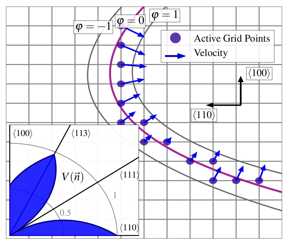
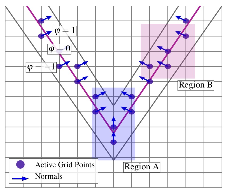
 with strong anisotropy (inset) cause spatially varying velocity values at active grid points. This effect is amplified at sharp corners of the front. As a consequence, from one time step to the other significant changes of the
effective at a specific grid point are induced. Since the level-set equation is hyperbolic, artificial waves of can be excited and subsequently propagated through the computational domain, which results in instable front propagation. (b) The topographies generated during typical SEG and anisotropic wet etching
simulations feature sharp corners (Region A) and extended flat surfaces (Region B).
with strong anisotropy (inset) cause spatially varying velocity values at active grid points. This effect is amplified at sharp corners of the front. As a consequence, from one time step to the other significant changes of the
effective at a specific grid point are induced. Since the level-set equation is hyperbolic, artificial waves of can be excited and subsequently propagated through the computational domain, which results in instable front propagation. (b) The topographies generated during typical SEG and anisotropic wet etching
simulations feature sharp corners (Region A) and extended flat surfaces (Region B).Reprinted with permission from Toifl et al., IEEE Access 8, 115406 [25] (2020). © 2020 Authors, licensed under the Creative Commons Attribution 4.0 License (http://creativecommons.org/licenses/by/4.0/).
In this section the incorporation of crystal orientation dependent etch or deposition rates into the level-set method is presented. As discussed in Section 2.2.5 and Section 3.2.2, a broad class of SEG
and anisotropic wet etching processes can be well-described with a distribution function which depends on the local surface normal vector  . Since is given by (4.11) it is a function of the spatial derivatives of :
  . Thus, the associated Hamiltonian is a function of the spatial derivatives:

A Hamiltonian constructed from an orientation-dependent velocity distribution is non-convex. If the surface has sharp corners, the non-convexity is problematic for the numerical stability of the discretized level-set equation [25], [119]. The reasons can be understood by considering an etch front with high
curvature, as illustrated in Fig. 4.3a. The profile is propagated with a non-convex numerical
Hamiltonian which originates from a velocity with possibly multiple extrema. As a consequence, the velocity assigned to the grid points is strongly varying, even for neighboring grid points. During front propagation the velocity between two grid points needs to be
estimated with some combination of the velocities exactly at these points [26]. The exact magnitude of the
velocity extrema and the placement of the front relative to the grid points are required for a high-quality estimation. However, this is difficult to achieve in a general setting. Furthermore, even if the global shape of the surface does
not significantly change after a small time step , the grid points near the surface are assigned a new set of considerably different velocities, hitting or missing the exact extrema of . As a result, the local advection speed can drastically change between time steps. Since the level-set equation (4.2) is a hyperbolic partial differential equation, locally confined sudden changes of values can excite numerical waves which spatially and temporally propagate through the computational domain. In a topography simulation, this highly undesired phenomenon can be observed as noisy and wavy
fronts in regions where a flat surface is expected.
Viscosity Solution
Anisotropic etch and growth simulations naturally involve sharp corners. Even in the continuous formulation of the level-set, a non-differentiable is required to resolve sharp corners, such as the V-shape displayed in Fig. 4.3b. As a
consequence, the physically expected solution of the level-set equation is not smooth. Thus, a more general methodology is required to solve (4.2), the so-called viscosity solution. The main idea of the viscosity solution is to add an artificial
viscosity term of the form  to the level-set equation (4.2). The adapted equation

asymptotically approaches the level-set equation for  . The vanishing viscosity allows to pick out the desired physical solution, which is a weak solution of the level-set equation. This is achieved by adding a diffusive component to (4.2) which also has a damping effect on waves that are excited by sudden changes of . Since the artificial viscosity is asymptotically vanishing, the method is called vanishing viscosity method. A further important benefit of this method is that viscosity solutions show reasonable behavior even if spatial
derivatives do not exist at isolated points in the domain (e.g., kinks or sharp corners) [16], [143].
. The vanishing viscosity allows to pick out the desired physical solution, which is a weak solution of the level-set equation. This is achieved by adding a diffusive component to (4.2) which also has a damping effect on waves that are excited by sudden changes of . Since the artificial viscosity is asymptotically vanishing, the method is called vanishing viscosity method. A further important benefit of this method is that viscosity solutions show reasonable behavior even if spatial
derivatives do not exist at isolated points in the domain (e.g., kinks or sharp corners) [16], [143].
Lax-Friedrichs Scheme
In order to apply the idea of the viscosity solution for the discretized level-set equation, the monotone Lax-Friedrichs scheme can be employed. This numerical scheme was originally introduced by Crandall and Lions [137] and is first-order in space. The characteristic feature is an additional linear numerical dissipation term. The Hamiltonian , as defined in (4.2), is replaced by the numerical Hamiltonian

at every active grid point  .
.  denotes the first-order forward/backward discretization of the spatial derivative with respect to
  and
and  are the dissipation coefficients. Hence, is composed of two terms

The first term is the finite difference discretization of the continuous Hamiltonian and the second term represents the numerical dissipation

The main idea of this scheme is to stabilize the surface propagation by adding numerical dissipation in regions of large spatial variations of . Fig. 4.3b shows a V-shaped front, where the region around the tip is characterized by high
curvature (Region A). Here, a large value of  is desired, while in flat regions (Region B), a small value of is sufficient to achieve stable front propagation. In order to achieve this behavior, the dissipation coefficients need to be appropriately defined. However, the calculation of is difficult in practice. If the respective values are too small, a noisy front materializes and propagating waves occur. On the contrary, if chosen too large, over-smoothing can arise, which results in overly rounded edges.
Multiple approaches to achieve stability and sharp geometrical features have been proposed. An elemental scheme which handles the case of spatially constant is [16]
is desired, while in flat regions (Region B), a small value of is sufficient to achieve stable front propagation. In order to achieve this behavior, the dissipation coefficients need to be appropriately defined. However, the calculation of is difficult in practice. If the respective values are too small, a noisy front materializes and propagating waves occur. On the contrary, if chosen too large, over-smoothing can arise, which results in overly rounded edges.
Multiple approaches to achieve stability and sharp geometrical features have been proposed. An elemental scheme which handles the case of spatially constant is [16]

where the maximum is taken for all points in a specific stencil  (thereby defining a Stencil Lax-Friedrichs scheme). If can be analytically described, appropriate dissipation coefficients can be directly derived [28].
However, an analytical form of for a general anisotropic wet etching and SEG process cannot be straight-forwardly formulated. Hence, the dissipation coefficients can either be heuristically chosen [118], or numerically approximated as proposed by Montoliu et al. [34].
Even though these approaches have been successfully employed for specific processes [120], they feature at least one numerical calibration parameter
which needs to be determined for every simulation configuration.
(thereby defining a Stencil Lax-Friedrichs scheme). If can be analytically described, appropriate dissipation coefficients can be directly derived [28].
However, an analytical form of for a general anisotropic wet etching and SEG process cannot be straight-forwardly formulated. Hence, the dissipation coefficients can either be heuristically chosen [118], or numerically approximated as proposed by Montoliu et al. [34].
Even though these approaches have been successfully employed for specific processes [120], they feature at least one numerical calibration parameter
which needs to be determined for every simulation configuration.
In the following section, a scheme is presented, which builds on these ideas and calculates in an optimized way for anisotropic processes. Most importantly, no heuristic parameters are required and thus allow for convenient application of numerically stable level-set based simulations for anisotropic wet etching
and SEG.
4.2 Stencil Lax-Friedrichs Scheme
A Stencil Lax-Friedrichs scheme for strongly anisotropic processes [25] is presented in this section. First, the scheme is rigorously derived from monotonicity considerations. Then, an implementation in ViennaTS is discussed and employed to analyze the capabilities of the scheme.
4.2.1 Derivation of the Scheme
As discussed in the previous section, the main idea of the Lax-Friedrichs scheme is to define a numerical Hamiltonian ((4.16) revisited)

which enables the convergence of the numerical solution of the level-set equation (4.2) to the viscosity solution. The time discretization ((4.4) revisited)

is the first-order forward Euler scheme. Crandall and Lions have established that the numerical Hamiltonian (4.16) with first-order spatial derivatives is stable if the scheme is monotone [137]. Thus, it is demanded that the scheme is non-decreasing in every argument  ,
,  ,
,  , and
, and  , where
  ,
,  , and
, and  refer to the grid point indices, corresponding to the three spatial coordinates. Applying these conditions to (4.4) and (4.16), results in four inequalities

Therefore, there are four conditions which need to be independently fulfilled on every grid point . The first inequality (4.20) relates the stable time step with the dissipation coefficients. Conditions (4.21) to (4.23) show that there is a lower limit for which is a function of  . This term cannot be geometrically interpreted, but incorporates the nature of the velocity function , e.g., the ratio of minimal and maximal velocity. In the case of a Hamiltonian which depends on the surface normal (4.14),
  with
with  can be further analyzed, because the components of the normal vector components
  can be expressed in terms of the spatial partial derivatives of

and has the form

In the following, the calculation of  is presented and the remaining expressions
  and
and  are derived analogously. First, the product rule of differentiation is applied

yielding two terms to consider. For the first term  the chain rule of differentiation is employed

The expressions  is evaluated by making use of (4.24)
![(4.28) \begin{equation} \frac {\partial V}{\partial \phi _x} = \frac {1}{\| \nabla \phi \|^3} \left [ \frac {\partial V}{\partial n^x} \left (\phi _y^2 + \phi _z^2\right ) - \frac
{\partial V}{\partial n^y} \phi _x \phi _y - \frac {\partial V}{\partial n^z} \phi _x \phi _z \right ]. \end{equation}](PhD_Thesis-images/image-404.svg)
The second term  is expressed in terms of

These intermediate results are applied to (4.26), which yields

Analogous calculations for and give rise to similar expressions and the general result can be expressed as

The term  can either be analytically (if possible) or numerically evaluated with a central difference scheme proposed by Montoliu et al. [34]

(and analogous terms for  and
and  ). A possible practical choice for
  is
is

with  referring to the floating point accuracy, which balances the truncation and round-off error [144].

consists of the grid point in question (center grid point) and all neighboring points (including diagonal neighbors). In a sparse-field level-set implementation, the set of active grid points is not sufficient to calculate the
dissipation coefficients of all neighboring points. Hence, the level-set values of grid points which are further away from the surface (  ) must be calculated in an expansion step (expanded grid points).
Reprinted with permission from Toifl et al., IEEE Access 8, 115406 [25] (2020). © 2020 Authors, licensed under the Creative Commons Attribution 4.0 License (http://creativecommons.org/licenses/by/4.0/).
(4.31) enables the practical consideration of conditions (4.21) to (4.23), which is used to define appropriate dissipation coefficients . These conditions only impose a lower limit on . Although there is no upper limit, large values of result in excessive dissipation which causes overly smooth numerical solutions of (4.2). As
a result, sharp edges are artificially rounded, which is not desired for the faceted topographies emerging during anisotropic processes. Hence, the coefficients are calculated based on the lower limit. Still, it is important to ensure that conditions (4.21) to (4.23) are fulfilled on every grid point , as required by the monotonicity criterion. A conservative technique to achieve this is to calculate the maximum of over the entire domain (referred to as Global Lax-Friedrichs scheme). However, since is essentially a local quantity, the maximum can also be calculated over a subset of , i.e., over a local stencil . In the extreme case consist only of one point, which is the point in question (referred to as Local Local Lax-Friedrichs) [16]. Only considering bears the risk of violating (4.21) to (4.23) in grid points near sharp edges.
Hence, a typical choice of involves a certain number of neighbor points (illustrated in Fig. 4.4), which motivates the
scheme for the calculation of dissipation coefficients for velocity distributions of the form 

The stencil consists of 9 and 27 grid points for 2D and 3D simulations, respectively, and includes the grid point and all neighboring grid points including diagonal neighbors. A trade-off between numerical stability and overly rounding of corners is achieved by considering local information with a rectangular stencil. If a small narrow
band or the sparse-field method is used, the calculation of the derivatives  potentially require -values outside the narrow band, or sparse field, respectively. Thus, an appropriate choice of the narrow band width or a dedicated expansion step in the case of the sparse-field method is required, which is indicated
in Fig. 4.4 by illustrating active and expanded grid points.
potentially require -values outside the narrow band, or sparse field, respectively. Thus, an appropriate choice of the narrow band width or a dedicated expansion step in the case of the sparse-field method is required, which is indicated
in Fig. 4.4 by illustrating active and expanded grid points.
In particular, the scheme (4.34) includes the term  , which is also present in the elemental scheme (4.19). In the case of spatially constant
 , (4.34) is reduced to the elemental scheme, and can thus be seen as an extension of the
elemental scheme. Furthermore, the inequality (4.20) connects the time step with . In order to fulfill this condition, the time step
, (4.34) is reduced to the elemental scheme, and can thus be seen as an extension of the
elemental scheme. Furthermore, the inequality (4.20) connects the time step with . In order to fulfill this condition, the time step  is calculated according to

where  refers to the narrow band or the set of active grid points (sparse-field method).
  is typically smaller than the time step indicated by the traditional CFL condition (4.10).
In summary, the Stencil Lax-Friedrichs scheme for surface normal dependent velocity distributions is defined as

First, the dissipation coefficients are calculated, then the time step is evaluated. These quantities are employed to define the numerical Hamiltonian as used in the first-order Euler time discretization of the level-set equation (4.2).
4.2.2 Implementation and Analysis
Fig. 4.5 shows a software flowchart of the steps required in a practical implementation of the Stencil Lax-Friedrichs
scheme, henceforth referred to as crystal anisotropy (CA) engine. The time loop controlling the front propagation during etching or deposition is visualized inside the blue box (solid lines). Compared to the general level-set
flow depicted in Fig. 4.2, the time loop is conceptually simpler. Since is assumed, the propagation velocity is not only defined on , but is actually a distributed quantity. This is a special property of the level-set method, because the normal vector can be calculated from the the level-set field with (4.11) and thus is well-defined in the entire
domain . Hence, no velocity extension is needed and the crystal rate model can be directly employed.

. The flow of operations is slightly simpler compared with Fig. 4.2, because velocity extension is not required. If a
SEG process is simulated, two additional steps (dashed lines) are performed. These involve the deposition top layer which is introduced in Section 4.3.
In order to asses the numerical capability of the scheme (4.36), a reference implementation of the CA
engine in ViennaTS has been developed [25]. Multiple material regions are described with multiple
level-set functions (which is further discussed in Section 4.3) and associated propagation velocities are assigned to
every material region. In order to enable the calculation of an expansion step is employed, where values in a larger vicinity of are calculated based on the sparse set of active grid points [118]. Stencils of active grid points are
partially overlapping, which is taken into account to calculate the dissipation coefficient for a specific active grid point only once per time step. The special case of active grid points located near a material boundary (e.g., interface between resist and substrate), is treated separately: Both material regions (  and
and  ) are assigned a dedicated velocity distribution,
  and
and  . If
. If  ,
,  is assumed for all velocity calculations needed for the Stencil Lax Friedrichs scheme (4.36).
Particular attention is required for grid points which are not located within one of the solid material regions, referred to as vacuum grid points in the following. These represent air or the surrounding atmosphere during a
fabrication process. In order to ensure continuous movement of , it is required that the level-set values on both sides of are evenly altered. This is achieved by assigning vacuum grid points adjacent to the velocity distribution of the material region on the other side of . This is generally implemented by determining the nearest solid material region, which is possible by inspecting the -values of all level-set functions describing all material regions.
Time Step Control
An important feature of the CA engine is the time step control (4.35), which ensures is consistent with with respect to the monotonicity requirement. But in a general simulation setting there are further constraints on . One is the CFL condition (4.10), which must be always fulfilled. Another constraint is present
in the case of etching of multiple material layers. Here, it is important to choose a time step  which ensures that a thin layer is not entirely traversed during one time step [118]. Thus, the
implementation in ViennaTS (independent of the Stencil Lax-Friedrichs scheme) first calculates
which ensures that a thin layer is not entirely traversed during one time step [118]. Thus, the
implementation in ViennaTS (independent of the Stencil Lax-Friedrichs scheme) first calculates

If anisotropic processes are simulated and the Stencil Lax-Friedrichs scheme (4.36) is employed, the final time step is

Analysis of Spatial Accuracy

 and depth of the V-tip
  are characteristic for a which has global minima at
  (one of the crystallographically equivalent minima is shown in the left image). An important geometry feature is the angle between substrate surface
  and
and  facets, which amounts to
  .
.Reprinted with adaptions from Toifl et al., IEEE Access 8, 115406 [25] (2020). © 2020 Authors, licensed under the Creative Commons Attribution 4.0 License (http://creativecommons.org/licenses/by/4.0/).


 in the Stencil Lax-Friedrichs scheme (4.36). The solid line represents the zero level-set of
the 2D wet etching experiment (Fig. 4.6). A uniform grid with parameter
in the Stencil Lax-Friedrichs scheme (4.36). The solid line represents the zero level-set of
the 2D wet etching experiment (Fig. 4.6). A uniform grid with parameter  is employed. (a) The dissipation coefficients
  and (b)
  are close to zero in flat regions, while they reach maximum values in proximity of the V-shaped corner. (c) Resulting numerical dissipation , which balances the artificially elevated values of the (d) Hamiltonian close to the corner. The resulting numerical Hamiltonian
  is characterized by small values for all active grid points. These values reflect the expected small etch rate imposed by
  . In particular, no locally elevated is present, which enables stable front propagation over time.
Reprinted with permission from Toifl et al., IEEE Access 8, 115406 [25] (2020). © 2020 Authors, licensed under the Creative Commons Attribution 4.0 License (http://creativecommons.org/licenses/by/4.0/).
In order to analyze the CA engine, a prototypical 2D anisotropic wet etching experiment previously encountered in Fig. 3.4 is considered and illustrated
in Fig. 4.6. The etch rate distribution of has the strongly anisotropic form depicted in the small inset figure (left) and the etch rate of the resist is assumed to be zero. The configuration is a demanding test for front propagation stability, because the mask
under-etching produces an etch front with sharp corners. Importantly, the etch front is expected to move with the slow etch rate associated with facets. Based on the 2D configuration the functional principle of the Stencil Lax-Friedrichs scheme (4.36) can be illustrated. Fig. 4.7a and Fig. 4.7b
visualize the dissipation coefficients and , as calculated in proximity to the V-shaped dip. and are approximately zero in flat regions, while they reach large values close to the sharp corner. The resulting dissipation term (Fig. 4.7c) balances the Hamiltonian (Fig. 4.7d), which is characterized by large values at sharp corners. Hence, the CA engine selectively adds the
appropriate amount of dissipation to in order to ensure a net surface propagation with consistently over the highly curved V-shaped dip.
The test configuration Fig. 4.6 allows for comparison of the simulation results with analytically calculated
geometric quantities. An etch rate distribution with global minimum for is assumed. As soon as facets are fully developed, the etch front is V-shaped and keeps this shape, while the mask undercut and the vertical position of the V-shaped tip linearly increases over time. If facets propagate in a geometrically ideal way with a rate , the values of these quantities are given by basic geometric relations

and

 is the angle between substrate surface and and amounts to
  . In order to quantify the accuracy of the simulated etch profile propagation, the simple error measure

(and the analogous  ) is used, which measures the accumulated error during an etch step of
  seconds duration. The simulated undercut and V-shape position are evaluated by extrapolating the etch profile lines and intersecting the lines with the mask- interface and with each other, respectively.
In the following, various etchants with rates given in Tab. 4.1 are investigated2. They have been labeled T1, T2, T3, KOH, SEG, whereby the latter two are typical representatives of rate anisotropy as encountered with the
etchants  and SEG techniques. Fig. 4.8 shows the simulated profiles for a 800 s etch process. The
homogeneous spatial resolution for all simulations is
and SEG techniques. Fig. 4.8 shows the simulated profiles for a 800 s etch process. The
homogeneous spatial resolution for all simulations is  and resulting geometric quantities and and error measures are given in Tab. 4.1. In all simulations (comprising more than 1000 time steps), the
accumulated relative error during the simulation is smaller than . Thus, the simulations with the CA engine provide excellent accuracy.
and resulting geometric quantities and and error measures are given in Tab. 4.1. In all simulations (comprising more than 1000 time steps), the
accumulated relative error during the simulation is smaller than . Thus, the simulations with the CA engine provide excellent accuracy.
and the corresponding simulation results for 2D 800 s wet etching simulation (Fig. 4.6). All have global etch rate minima at and thus are inducing the characteristic V-shaped profile. The simulated mask undercut and the V tip shift compared with the ideal values  . These values reflect the change in topography between the initial time
  and
and  . In the case of the SEG etchant, the V-shaped profile is not fully evolved before
  , in all other cases
  . The spatial resolution for all simulations is and the resulting profiles are depicted in Fig. 4.8.
Reprinted with permission from Toifl et al., IEEE Access 8, 115406 [25] (2020). © 2020 Authors, licensed under the Creative Commons Attribution 4.0 License (http://creativecommons.org/licenses/by/4.0/).
| Rates (µm/min) | Etch Times (s) | Distances (µm) | Relative Error | |||||||||
| Etchant |  |
 |
|
 |
|
|
|
 |
|
 |
 |
|
| KOH | 1.0 | 1.855 | 0.0073 | 1.801 | 800 | 0 | 0.122 | 0.119 | 0.172 | 0.169 | 0.587 | 0.830 |
| SEG | 0.5 | 0.2 | 0.05 | 0.25 | 800 | 83 | 0.732 | 0.731 | 1.035 | 1.033 | 0.321 | 0.321 |
| T1 | 1.0 | 1.5 | 0.03 | 1.5 | 800 | 0 | 0.488 | 0.490 | 0.691 | 0.693 | 0.328 | 0.463 |
| T2 | 1.0 | 0.6 | 0.05 | 0.9 | 800 | 0 | 0.815 | 0.816 | 1.152 | 1.155 | 0.392 | 0.554 |
| T3 | 0.7 | 0.6 | 0.04 | 1 | 800 | 0 | 0.655 | 0.653 | 0.926 | 0.924 | 0.388 | 0.549 |
The high accuracy is enabled by the inclusion of the additional terms in calculation of (see (4.34)). Fig. 4.9a and Fig. 4.9b demonstrate that the elemental scheme (4.19) results in wavy etch profiles and unacceptably errors . In contrast, the Stencil Lax-Friedrichs scheme (4.36) stabilizes the front propagation, as
evident from flat facets and the congruence with the ideal profile. Furthermore, the magnitude of the associated relative errors of the elemental scheme strongly depends on the etch rate distribution , as indicated by the significantly larger error observed with etchant KOH compared to etchant SEG.

and the spatial resolution is . The geometries display the characteristic planes, which form a V-shaped profile. All distances are given in  .
.Reprinted with adaptions from Toifl et al., IEEE Access 8, 115406 [25] (2020). © 2020 Authors, licensed under the Creative Commons Attribution 4.0 License (http://creativecommons.org/licenses/by/4.0/).
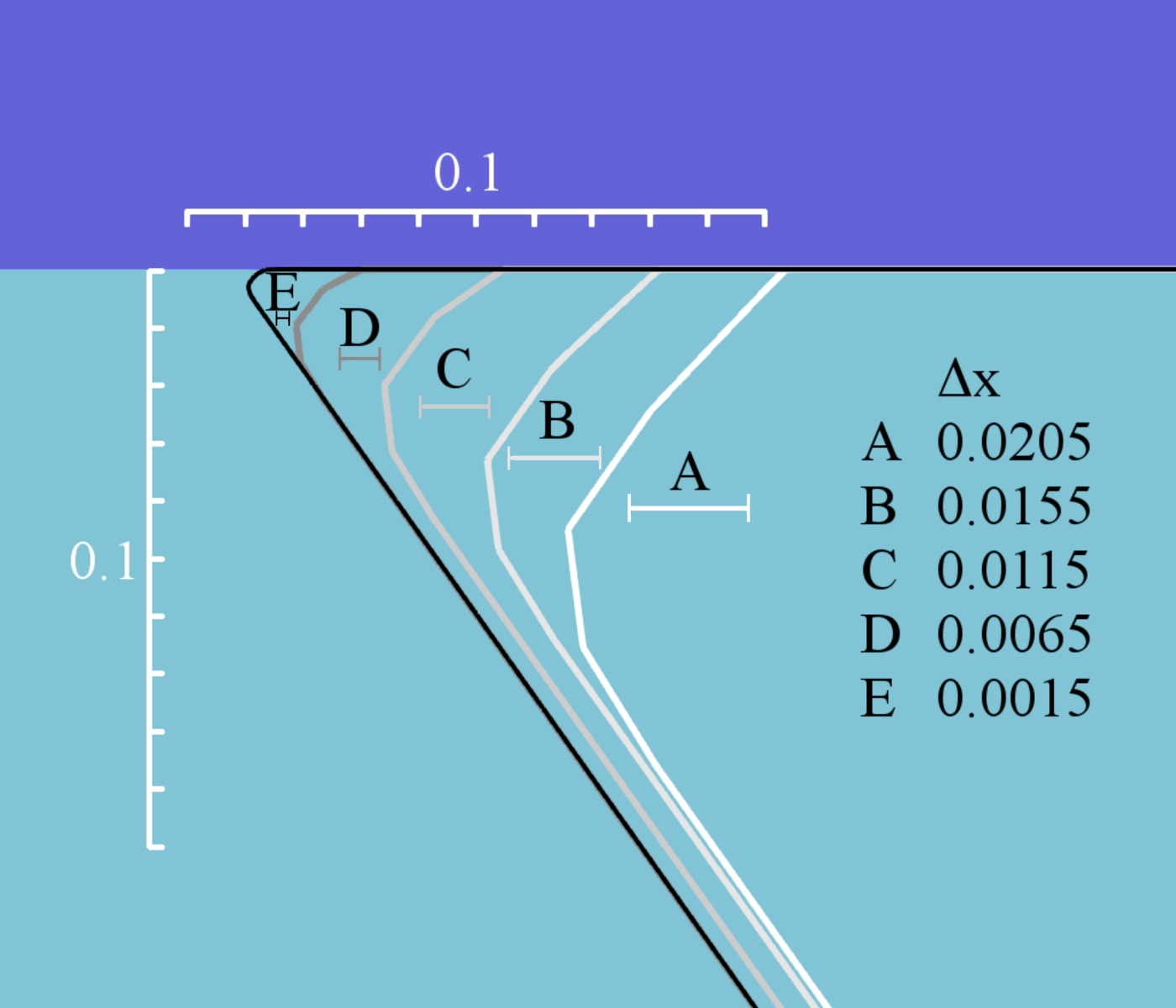
Even though the Stencil Lax-Friedrichs scheme stabilizes the front propagation, the dissipation term introduces rounding to sharp corners. The reference wet etching simulation also allows for quantification of the rounding effect by
studying the etch front directly beneath the mask. Fig. 4.9c shows the simulation results for different spatial
resolutions ranging from ![\( \Delta x = \num [round-mode=places,round-precision=4]{0.0205} \)](PhD_Thesis-images/326E67519F939BB5661D2CBBD8120EF2.svg) to
to ![\( \Delta x = \num [round-mode=places,round-precision=4]{0.0015} \)](PhD_Thesis-images/9DECDF361C238564E65FB093315D0F20.svg) . The Stencil Lax-Friedrichs scheme (4.36) causes rounding extending over roughly three
grid cells, which also is the case for
. The Stencil Lax-Friedrichs scheme (4.36) causes rounding extending over roughly three
grid cells, which also is the case for  .
.


 is employed, the propagation is instable and results in noisy fronts (label B), even though the advanced adaptive time stepping (4.35)
is used. By contrast, the Stencil Lax-Friedrichs scheme (4.34) enables high accuracy fronts (label
A). The magnitude of the error strongly depends on the etchant. (c) Rounding extending over approximately three grid spacings is introduced by the Stencil Lax-Friedrichs scheme, which is a general feature of
Lax-Friedrichs schemes due to the added dissipation terms. All distances are given in .
is employed, the propagation is instable and results in noisy fronts (label B), even though the advanced adaptive time stepping (4.35)
is used. By contrast, the Stencil Lax-Friedrichs scheme (4.34) enables high accuracy fronts (label
A). The magnitude of the error strongly depends on the etchant. (c) Rounding extending over approximately three grid spacings is introduced by the Stencil Lax-Friedrichs scheme, which is a general feature of
Lax-Friedrichs schemes due to the added dissipation terms. All distances are given in .Reprinted with adaptions from Toifl et al., IEEE Access 8, 115406 [25] (2020). © 2020 Authors, licensed under the Creative Commons Attribution 4.0 License (http://creativecommons.org/licenses/by/4.0/).
2 The continuous distributions are constructed via (trilinear) Hubbard interpolation [145], as further discussed in Section 5.1.
Analysis of Time Stepping
The time step control (4.35) is essential for the stabilization of front propagation. In the following
the impact of the time step reduction is investigated by comparing the results of simulations employing the traditional and the Stencil Lax-Friedrichs time step control. In the latter case, there is no associated intrinsic CFL
parameter and simulations are performed with the maximum CFL value for the sparse field method, i.e., ![\( C_\mathrm {CFL} = \num [round-mode=places,round-precision=1]{0.5} \)](PhD_Thesis-images/0D30502D4DD32E4ABAAA13B32925139B.svg) [118]. With this choice only the active grid points can change the sign of the level-set value during
one time step, thus enabling robust front propagation. In the traditional case, different values for
[118]. With this choice only the active grid points can change the sign of the level-set value during
one time step, thus enabling robust front propagation. In the traditional case, different values for  in the range from
  to
to  are employed. Smaller values imply smaller time steps . The impact of etchant, spatial resolution, and on the accuracy of the front propagation is demonstrated in Tab. 4.2, where again a
  etching simulation (Fig. 4.6) is considered. In particular, the nature of is significant for the time stepping. The traditional time step calculation requires a CFL number of 0.01 for etchant KOH to fulfill the high accuracy criterion
  .
.  is sufficient for excellent accuracy in the case of etchant SEG, while etchant T2 requires
  for highly accurate results. Therefore, in order to achieve high-quality simulation results the appropriate
  needs to be known a priori, which is not the case for general etchants.
and , respectively) for 2D simulations of 800 s wet etching. The results obtained from time stepping employing different CFL numbers and from advanced adaptive time stepping (4.41). Entries indicated with  refer to simulations where the front drifted out of the simulation domain (caused by severe instable front propagation). The relative error depends significantly on the employed and is particularly high for etchant KOH. Here, extremely small time steps need to be enforced by small CFL numbers to achieve
  .
.Reprinted with permission from Toifl et al., IEEE Access 8, 115406 [25] (2020). © 2020 Authors, licensed under the Creative Commons Attribution 4.0 License (http://creativecommons.org/licenses/by/4.0/).
| Distances (µm) | Relative Error | ||||
| Etchant | |
|
|
|
 |
| KOH | 0.5 | |
|
|
|
![\( \Delta x = \num [round-mode=places,round-precision=4]{0.0105} \)](PhD_Thesis-images/5C53CE1CC1DAED6A2C02B13A76BC6C66.svg) |
0.3 | 0.611 | 0.886 | 46.850 | 68.280 |
| 0.1 | 0.247 | 0.353 | 12.153 | 17.519 | |
| 0.05 | 0.133 | 0.189 | 1.356 | 1.918 | |
| 0.03 | 0.135 | 0.191 | 1.543 | 2.182 | |
| 0.01 | 0.122 | 0.173 | 0.295 | 0.421 | |
| Adaptive | 0.118 | 0.166 | 0.159 | 0.225 | |
| Ideal | 0.119 | 0.169 | |||
| KOH | 0.5 | |
|
|
|
![\( \Delta x = \num [round-mode=places,round-precision=4]{0.0045} \)](PhD_Thesis-images/38DBE59B9482B330131251F30703919B.svg) |
0.3 | 0.622 | 0.905 | 111.703 | 163.577 |
| 0.1 | 0.195 | 0.278 | 16.893 | 24.245 | |
| 0.05 | 0.154 | 0.218 | 7.695 | 10.883 | |
| 0.03 | 0.134 | 0.190 | 3.268 | 4.719 | |
| 0.01 | 0.122 | 0.174 | 0.527 | 1.161 | |
| Adaptive | 0.122 | 0.172 | 0.587 | 0.830 | |
| Ideal | 0.119 | 0.169 | |||
| Distances (µm) | Relative Error | ||||
| Etchant | |
|
|
|
|
| SEG | 0.5 | 0.732 | 1.036 | 0.070 | 0.220 |
| |
0.3 | 0.731 | 1.035 | 0.030 | 0.160 |
| 0.1 | 0.731 | 1.035 | 0.001 | 0.110 | |
| 0.05 | 0.731 | 1.035 | 0.001 | 0.110 | |
| 0.03 | 0.731 | 1.034 | 0.010 | 0.100 | |
| 0.01 | 0.731 | 1.034 | 0.010 | 0.100 | |
| Adaptive | 0.731 | 1.036 | 0.060 | 0.200 | |
| Ideal | 0.731 | 1.039 | |||
| T2 | 0.5 | |
|
|
|
| |
0.3 | 0.986 | 1.446 | 46.308 | 75.069 |
| 0.1 | 0.815 | 1.152 | 0.512 | 0.695 | |
| 0.05 | 0.814 | 1.151 | 0.877 | 0.532 | |
| 0.03 | 0.814 | 1.151 | 0.881 | 1.246 | |
| 0.01 | 0.814 | 1.151 | 0.884 | 1.250 | |
| Adaptive | 0.815 | 1.152 | 0.392 | 0.554 | |
| Ideal | 0.816 | 1.155 | |||
In contrast, results originating from Stencil Lax-Friedrichs control (4.35) (also referred to as
advanced adaptive time stepping, and denoted as Adaptive in Tab. 4.2), show high accuracy. In order to
investigate the reasons for the high accuracy, the individual steps are observed during the test simulation. Fig. 4.10a shows a histogram of associated with the etchant KOH. The traditional implementation with  and the time step control (4.35) result in significantly different distributions. A broad
distribution of with two distinctive peaks can be observed with the traditional implementation, while the adaptive scheme exhibits a significantly narrower distribution. The progression of over time is illustrated in Fig. 4.10b, indicating strong fluctuations in in the traditional scheme. These can be attributed to the non-convex nature of the Hamiltonian, which causes fluctuations in the velocities assigned to active grid points. As a consequence, the maximum velocity
and thus (4.37) depends on the position of the front relative to the grid, which causes variations in spanning more than three orders of magnitude.
and the time step control (4.35) result in significantly different distributions. A broad
distribution of with two distinctive peaks can be observed with the traditional implementation, while the adaptive scheme exhibits a significantly narrower distribution. The progression of over time is illustrated in Fig. 4.10b, indicating strong fluctuations in in the traditional scheme. These can be attributed to the non-convex nature of the Hamiltonian, which causes fluctuations in the velocities assigned to active grid points. As a consequence, the maximum velocity
and thus (4.37) depends on the position of the front relative to the grid, which causes variations in spanning more than three orders of magnitude.
In both implementations the structural change of the topography from the initial geometry to fully emerged facets is reflected in the magnitude of . Before the V-shaped profile is formed (  in Fig. 4.6), constant small time steps are employed in the traditional case, but as soon as the etch front
slowly undercuts the mask, fluctuations in maximum velocity arise. These cannot be resolved by reducing to considerably small values, as the root cause of the fluctuations is not resolved. In contrast, the advanced adaptive time stepping strongly reduces the fluctuation of , indicating that the front is numerically stable. A further observation is a periodic pattern starting at
in Fig. 4.6), constant small time steps are employed in the traditional case, but as soon as the etch front
slowly undercuts the mask, fluctuations in maximum velocity arise. These cannot be resolved by reducing to considerably small values, as the root cause of the fluctuations is not resolved. In contrast, the advanced adaptive time stepping strongly reduces the fluctuation of , indicating that the front is numerically stable. A further observation is a periodic pattern starting at  , which can be attributed to repeatedly occurring relative alignment of the front with respect to the grid.

 in 800 s wet etching simulations (KOH,
  ). denotes the total number of time steps. The traditional time stepping (top) employs a small , which enables results of acceptable accuracy (quantified by the high accuracy criterion , as presented in Tab. 4.2). The associated histogram shows a broad distribution of with two distinctive peaks. By contrast, the advanced adaptive time stepping (bottom) results in a narrow distribution. (b) Temporal evolution of for the first 500 s. The traditional time stepping (top) exhibits oscillations which originate from strongly varying velocity values in the proximity of the V-shaped corner. In contrast, the advanced adaptive time
stepping (bottom) reduces the time step in case high values of dissipation are needed.
). denotes the total number of time steps. The traditional time stepping (top) employs a small , which enables results of acceptable accuracy (quantified by the high accuracy criterion , as presented in Tab. 4.2). The associated histogram shows a broad distribution of with two distinctive peaks. By contrast, the advanced adaptive time stepping (bottom) results in a narrow distribution. (b) Temporal evolution of for the first 500 s. The traditional time stepping (top) exhibits oscillations which originate from strongly varying velocity values in the proximity of the V-shaped corner. In contrast, the advanced adaptive time
stepping (bottom) reduces the time step in case high values of dissipation are needed.Reprinted with permission from Toifl et al., IEEE Access 8, 115406 [25] (2020). © 2020 Authors, licensed under the Creative Commons Attribution 4.0 License (http://creativecommons.org/licenses/by/4.0/).
The analysis presented in this section demonstrates that the CA engine provides the capability to simulate front propagation under strongly anisotropic with high accuracy. In the next section, multi-material configurations are discussed. These are particularly important for non-planar SEG.
4.3 Multi Level-Set Scheme for Non-Planar Selective Epitaxy
Semiconductor device structures consist of multiple materials which are shaped during fabrication processes. A strategy to incorporate multiple material regions into the level-set method is to use a multi-level-set approach. Each material region is represented by a level-set function, resulting in a set of level-set functions. Robust handling of material interfaces is essential and can be achieved with an additive enclosure technique, which is referred to as layer wrapping.
The level-set layer  representing a specific material region
  is described by the boundary surface of the union of all underlying material regions

Therewith all material regions in are described with a stack of level-set functions. In order to construct the enclosing layers set operations (Boolean operations) are employed. These can be conveniently expressed in the level-set framework [136], as shown by two example correspondences of geometric and level-set operations for union and complement

where a level-set function  describes the boundary
  . The level-set operations are applied pointwise for all grid points. Thus, (4.42) can be directly
expressed in terms of the level-set functions. A special role plays the topmost layer
. The level-set operations are applied pointwise for all grid points. Thus, (4.42) can be directly
expressed in terms of the level-set functions. A special role plays the topmost layer  , the so-called top layer. Since
  describes the exposed features of the multi-material stack, it is subjected to the fabrication process. Hence, the corresponding level-set function
  is propagated according to the velocity model . The underlying layers
  are typically not affected and the associated level-set values
  remain constant. Only in special cases, such as etching through multiple material regions, are updated accordingly to maintain the consistency of the construction (4.42) [118].
The highly anisotropic models associated with anisotropic wet etching and SEG processes result in high sensitivity on the local surface normal vector. Thus, an accurate description of the zero level-set of is necessary. The additive multi-level-sets approach is well-suited for etching simulations. However, it is not suitable for selective growth processes, because for some configurations the local convexity is artificially altered
at material interfaces. In Fig. 4.11 corner regions are highlighted (white circles), where ,  , and SiGe material regions coincide. These are problematic for selective deposition simulation, because the top layer, as constructed with (4.42), imposes a concave level-set, even though the newly deposited SiGe forms a convex geometry. As a
result, inaccuracies of the local surface normal vector due to the discretization of level-set function strongly affect the surface evolution. The growth simulation shown in Fig. 4.11 illustrates that these inaccuracies cause non-symmetrical topographies, even though the initial trench structure is
perfectly symmetric. In order to circumvent these inaccuracies, the deposition top layer method which employs Boolean operations to construct a specialized top layer is introduced in the following section.
, and SiGe material regions coincide. These are problematic for selective deposition simulation, because the top layer, as constructed with (4.42), imposes a concave level-set, even though the newly deposited SiGe forms a convex geometry. As a
result, inaccuracies of the local surface normal vector due to the discretization of level-set function strongly affect the surface evolution. The growth simulation shown in Fig. 4.11 illustrates that these inaccuracies cause non-symmetrical topographies, even though the initial trench structure is
perfectly symmetric. In order to circumvent these inaccuracies, the deposition top layer method which employs Boolean operations to construct a specialized top layer is introduced in the following section.

 ,
,  ,
,  ,
,  ,
,  ,
,  , and
, and  ; ).
; ).Reprinted with adaptions from Toifl et al., IEEE Access 8, 115406 [25] (2020). © 2020 Authors, licensed under the Creative Commons Attribution 4.0 License (http://creativecommons.org/licenses/by/4.0/).
4.3.1 Deposition Top Layer

 , but not on the oxide. (a) The traditional initial top layer
  circumscribes and oxide, while the deposition top layer
  does not include the oxide. Additionally, the orientation is flipped, which ensures consistent orientation of
  and the mask. (b) enables robust growth and subsequently, the final deposition top layer
  is converted back to the traditional representation
  by applying Boolean operations (4.47).
Reprinted with permission from Toifl et al., IEEE Access 8, 115406 [25] (2020). © 2020 Authors, licensed under the Creative Commons Attribution 4.0 License (http://creativecommons.org/licenses/by/4.0/).
The artifacts in local surface normals at multi-material interfaces can be prevented by adapting the top layer construction. Prior to a deposition step, the initial top layer is divided into two subsets. The first subset consists of all material regions with a non-zero growth rate and is denoted as  (referring to epitaxial growth). The second subset is the union of material regions with zero growth rate. In a typical simulation this is the set of masks, and thus is referred to as mask

The initial deposition top layer is constructed as

where denotes the computational domain. Fig. 4.12a illustrates the conventional and deposition top layer for a
fin structure. While the conventional construction encompasses the fin and , is only wrapped around the fin. Additionally, the orientation of level-set function is inverted, as indicated with arrows. The change of orientation ensures that and are consistently orientated for growing . A consequence of the orientation flipping is that the growth distribution used for surface propagation also needs to be inverted  . At the end of the deposition step, the deposition top layer has the final geometry . In order to transition back to the conventional top layer, a conversion step is performed

which is also based on aggregated union and complement operations. Fig. 4.12b visualizes the final topography and the associated layers.
The implementation of the deposition top layer is discussed in the next section, where also its capability and suitability is analyzed.
4.3.2 Implementation and Analysis

, , , , , , and ; ).Reprinted with adaptions from Toifl et al., IEEE Access 8, 115406 [25] (2020). © 2020 Authors, licensed under the Creative Commons Attribution 4.0 License (http://creativecommons.org/licenses/by/4.0/).
The deposition top layer approach is an addition to the CA engine. As indicated in the flowchart of Fig. 4.5, the conversion to the deposition top layer and the back conversion are applied only in the case of selective deposition. The front propagation proceeds with the Stencil Lax-Friedrichs scheme (4.36) in the same way as in the anisotropic wet etching case. Thus, the only difference are two additional Boolean operation steps per selective deposition process. In order to implement the conversion from the traditional top layer to the deposition top layer, the entire material stack has to be considered.
Deposition Top Layer Algorithm
An algorithm which constructs the mask subset based on the selectivity of deposition process is presented in Algorithm 1. The term selectivity refers here to the capability of a material region to have impinging species deposited. For
example, in a SiGe SEG process, epitaxial SiGe is grown on top of , but not on top of . In this case the material region associated with SiGe is a deposition substrate in the nomenclature of Algorithm 1, while is not. Therewith, the entire material stack is characterized with a list  (DepositionPossible) storing whether
  is a deposition substrate. The back-conversion from
  to is achieved by directly employing (4.47) with the Boolean operations given in (4.43).
Algorithm 1: Algorithm to calculate the level-set value of the deposition top layer for a specific grid point. stores which material regions constitute a so-called deposition substrate, i.e., a material region where SEG can occur.  refers to the upper limit of values, typically determined by the width of the narrow band.
Data: DepositionPossible
list ,
multi-layer level-set list  ,
,
level-set value at grid point
Result: Deposition
top layer
 //
//  of upper layer


if not all layers are deposition substrate then


else

end
 // Invert layer
orientation
// Invert layer
orientation
With the deposition top layer, the inaccuracies in multi-material simulations are resolved, as demonstrated in Fig. 4.13. The initial deposition top layer is a horizontal line in this case and is indicated with a white dashed line. Most importantly, does not enforce a concave surface, on the emerging SiGe region. The SiGe film, as described by the deposition top layer, is propagated correctly and the symmetry of the initial trench is respected.

 which results in the formation of facets. All distances are given in .
Reprinted with adaptions from Toifl et al., IEEE Access 8, 115406 [25] (2020). © 2020 Authors, licensed under the Creative Commons Attribution 4.0 License (http://creativecommons.org/licenses/by/4.0/).
Analysis
In the following, the CA engine for SEG, which is comprised of the deposition top layer and Stencil-Lax-Friedrichs scheme, is assessed by considering the 3D structure in Fig. 4.14a, which consists of a cuboidal fin surrounded by a film. During SEG a large SiGe crystal is formed with characteristic facets (Fig. 4.14b). Similar to the 2D anisotropic wet etching configuration discussed in Section 4.2.2, ideal distances can be expressed in terms of and thus employed as a benchmark for assessing the quality of simulation results achieved with the CA engine. The lateral distance is given by

where  . The ideal overgrowth height
  can be expressed in terms of
  and the fin length

These relations are valid if the growth function has its global minimum at directions and as soon as all have fully emerged. Fig. 4.15 shows two slices of the 3D growth simulation at different process times: One
perpendicular to the Si fin (Fig. 4.15a) and one along the fin (Fig. 4.15b). In the early stages of the growth, are gradually dominating the topography until they are fully emerged at  . Subsequently, the lateral growth occurs with rate of approximately
  . At
. At  the simulated lateral distance
  , yielding a relative spatial error of
  . The simulated overgrowth height
  is 0.021 µm. Additionally, the quality of the simulated planes is assessed by comparing the angles
  and
and  , as illustrated in Fig. 4.15, with the angles between the ideal crystallographic facets. As presented in
Tab. 4.3, the results show high accuracy of the simulated facets.
, as illustrated in Fig. 4.15, with the angles between the ideal crystallographic facets. As presented in
Tab. 4.3, the results show high accuracy of the simulated facets.
4.4 Summary
 and
and  planes, while ideal distances are calculated using (4.48) and ([25] (2020). © 2020
Authors, licensed under the Creative Commons Attribution 4.0 License (http://creativecommons.org/licenses/by/4.0/).
planes, while ideal distances are calculated using (4.48) and ([25] (2020). © 2020
Authors, licensed under the Creative Commons Attribution 4.0 License (http://creativecommons.org/licenses/by/4.0/).
| Angles (°) | Distances (µm) | |||||
 |
 |
 |
 |
 |
|
|
| Ideal | 109.5 | 70.53 | 125.3 | 54.74 | 0.0102 | 0.0215 |
| Simulated | 109.5 | 70.53 | 125.3 | 54.73 | 0.010 | 0.020 |


 ( , ,
( , ,  ,
,  , and
, and  ). The angles indicated with , , , and are compared with the ideal values in Tab. 4.3.
Reprinted with adaptions from Toifl et al., IEEE Access 8, 115406 [25] (2020). © 2020 Authors, licensed under the Creative Commons Attribution 4.0 License (http://creativecommons.org/licenses/by/4.0/).
The CA engine proposed in this thesis, enables stable and robust level-set method simulations of anisotropic wet etching and selective deposition. The underlying Stencil Lax-Friedrichs discretization scheme originates from monotonicity considerations and provides optimized front propagation for normal-dependent etch and growth models. This is achieved by constructing a first-order monotone scheme to discretized the level-set equation which is of the Hamilton-Jacobi type. In particular, monotonicity criteria are applied to determine stability-enabling time steps and dissipation coefficients of the Lax-Friedrichs scheme. In contrast to previous studies [34], the developed scheme presented in this chapter does not require heuristic numerical factors, which significantly facilitates the model development process. Although the implementation discussed in this chapter is based on the sparse-field level-set method, is can also be directly incorporated into narrow-band based level-set frameworks by implementing (4.36).
Furthermore, the deposition top layer method, which is a multi level-set configuration to enable robust selective epitaxy simulations, was proposed. The deposition top layer method is based on Boolean operations and avoids the artificial introduction of incorrect convexity, which is particularly detrimental in trench configurations.
In the following chapter, the CA engine is applied to simulate several wet etching and SEG configurations. Furthermore, developed models are introduced for different crystal symmetries and process conditions.