Only carriers with high energies contribute to the avalanche process. Like all high-energy mechanisms, impact-ionization is a non-local process (compare Section 4.3.1). This leads to problems in classical drift-diffusion simulation environments, because only local quantities are available, while no exact information on the distribution function can be obtained. Also hydrodynamic simulations deliver only the mean energy. Thus, the information on high-energy tails of the carrier distribution function is not available (see Section 4.3.2). As a result, drift-diffusion and/or hydrodynamic schemes require modeling approaches which are only based on local quantities.
In drift-diffusion simulations, the only local quantity that allows conclusions on the
carrier temperature and therefore on the impact-ionization rate is the electric field. Many
authors who investigated the ionization coefficients, both, experimentally and
theoretically, suggested an exponential relation to the electric field ![]() as
[11]
as
[11]
An early approach deriving the value of the parameter ![]() from the BTE
was performed by Baraff [195]. He showed that the different values
1 and 2 used for
from the BTE
was performed by Baraff [195]. He showed that the different values
1 and 2 used for ![]() are the limiting cases for relatively low and
high fields. However, there is no closed solution of his approach, but
approximations have been presented in various publications, for example, by
Crowell et al. [196],
are the limiting cases for relatively low and
high fields. However, there is no closed solution of his approach, but
approximations have been presented in various publications, for example, by
Crowell et al. [196],
Another local-field model was presented by Lackner [198], who derived an expression which leads to an extension of Chynoweth's law,
 |
(5.15) |
 |
(5.16) |
Slotboom et al. [199] have observed lower impact ionization rates for currents near the surface. As a consequence, models describing the transition between surface and bulk impact ionization have been developed [200]. However, Monte Carlo simulations have shown that there are no or only minor differences between surface and bulk impact ionization rates [201]. This means that there is no physical evidence of different rates near the surface and that those models are based on artifacts resulting from the approximate ionization rates based on the electric field.
In many applications, local-field based models deliver good results. However, from the physical point of view, impact-ionization is not field dependent. This is especially important in areas of rapidly changing electric fields and in small devices. This weakness can be observed in Fig. 5.4 for a 200nm and a 50nm structure. This figure compares generation rates calculated using different transport schemes. In this example, the electrons are accelerated from left to right. As soon as the electric field is risen, the local-field model predicts the carrier generation rate. However, physically more correct are the Monte Carlo reference simulations. They demonstrate that the carrier energy can follow changes in the electric field with a certain delay. At characteristic lengths shown in that figure, the validity of the local-field approach becomes questionable.
As long as device expansions are well above ![]() nm, the advantages of
local-field models are the good integrability in drift-diffusion schemes which are the
workhorse in device simulation tools. Most TCAD simulators therefore commonly
include one or more of the local electric field models. A typical application
where drift-diffusion models deliver good results are high-voltage LDMOS
transistors. Fig. 5.5 shows some results based on
(5.13) and also clearly shows the importance of this
physical effect. A more comprehensive example incorporating breakdown and
snap-back simulations is presented in Section 5.3.
nm, the advantages of
local-field models are the good integrability in drift-diffusion schemes which are the
workhorse in device simulation tools. Most TCAD simulators therefore commonly
include one or more of the local electric field models. A typical application
where drift-diffusion models deliver good results are high-voltage LDMOS
transistors. Fig. 5.5 shows some results based on
(5.13) and also clearly shows the importance of this
physical effect. A more comprehensive example incorporating breakdown and
snap-back simulations is presented in Section 5.3.
Local modeling approaches do not provide information about where carriers come
from and if they have already gained high energy. But since electrons and holes
have to be accelerated to gain at least the threshold energy before impact-ionization can
occur, this information is relevant. The area where there is a high electric
field but impact-ionization has not started yet is often called dark-space
[202]. This dark-space has to be considered also in experimental
extractions of the ionization coefficients. Measuring of the coefficients
cannot be performed directly. Therefore, they are commonly extracted out of the
multiplication factor using the ionization integral
(5.10). While considering the dark-space, the boundaries
of the ionization integral are shifted so that only regions where impact-ionization takes
place are included. With this approximation Okuto and Crowell [202]
could explain anomalous energies which were found previously for the parameters
![]()
![]() and
and ![]() in (5.14). They have obtained more
realistic energies employing a pseudo-local approximation which is also valid
for high fields. In their work, a model using apparent and real
ionization coefficients was developed. This technique delivered reasonable
results for the given one-dimensional examples.
in (5.14). They have obtained more
realistic energies employing a pseudo-local approximation which is also valid
for high fields. In their work, a model using apparent and real
ionization coefficients was developed. This technique delivered reasonable
results for the given one-dimensional examples.
An interesting approach which includes local changes of the electric field is the method presented by Slotboom et al. [179] (compare (4.23)). The required post-processing which is necessary after a conventional drift-diffusion simulation, makes this method elaborative to implement, especially if self-consistent solutions are required.
The lucky electron concept [192,203] introduces a threshold
energy level
![]() The carriers need to surmount this
potential barrier in order to trigger impact-ionization. Hu et al. [203] describes that
this energy can be reached if a carrier travels a sufficiently long distance
without collisions. In this work by Hu, a compact model is formulated, which
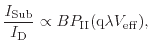
relates the substrate current
The carriers need to surmount this
potential barrier in order to trigger impact-ionization. Hu et al. [203] describes that
this energy can be reached if a carrier travels a sufficiently long distance
without collisions. In this work by Hu, a compact model is formulated, which
relates the substrate current
![]() as a consequence of impact-ionization with the drain
current
as a consequence of impact-ionization with the drain
current
![]() and the maximum electric field
and the maximum electric field
![]() in the device. The drain
current acts as a source function (the supply of carriers) and the peak field
is used together with the (hot-carrier) mean free path
in the device. The drain
current acts as a source function (the supply of carriers) and the peak field
is used together with the (hot-carrier) mean free path ![]() to describe
the ionization probability. This leads to
to describe
the ionization probability. This leads to
A method to utilize the lucky electron model in device simulation and to
introduce the non-locality has been proposed by
Meinerzhagen [205]. In this work, the electric field line is
followed starting from a point ![]() until the electrostatic potential difference
of
until the electrostatic potential difference
of
![]() has been reached at a point
has been reached at a point ![]() The length
along the field line between
The length
along the field line between ![]() and
and ![]() is
is ![]() The generation rate in the
point
The generation rate in the
point ![]() yields
yields
 |
(5.18) |
Another approach for modeling impact-ionization employs the carrier temperature, i.e. the
local mean carrier energy, as the key parameter. The formalism for the rate
calculation is very similar to the local-field model. For the transformation of
the commonly used local field based models, the electric field can be replaced
by the homogenous stationary energy balance equation, compare
(4.19), to form
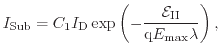
![]() [206]. Thus, Chynoweth's law can be transformed from
(5.13) to a carrier temperature dependent model. An often
used estimation combining all coefficients reads [207]
[206]. Thus, Chynoweth's law can be transformed from
(5.13) to a carrier temperature dependent model. An often
used estimation combining all coefficients reads [207]
|
|
It seems natural to use the carrier energy in place of the electric field to model the impact-ionization rate and it is commonly used in the energy-transport or hydrodynamic simulation frameworks. Hence, it is possible to approximately consider non-local issues like the dark-space phenomenon. However, the carrier temperature alone cannot reflect the existence and strength of high-energy tails, i.e. the amount of high energetic carriers available. Completely different shapes of the distribution function can lead to the same average energy [15]. Additionally, high-energy tails can also exist if the average energies are low (compare Fig. 4.2 and 4.12). Therefore, the carrier temperature is commonly overestimated in small devices, which also leads to an overestimation of the impact-ionization rate [208,186]. These effects, which are especially relevant for aggressively down-scaled devices, can only be considered by incorporating the full distribution function.
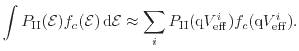
Instead of using the electric field, the carrier temperature, hot-carrier
sub-populations, or some non-local approximations, the most rigorous modeling
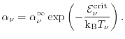
approach is to directly incorporate the carrier distribution function
![]() This allows one to calculate the total generation rate
using [187]
This allows one to calculate the total generation rate
using [187]
The integration boundaries in (5.20) show that only carriers
above a certain energy threshold
![]() influence the generation rate and
highlight that high energies are of vital importance. Approximations of the
distribution function based on splitting hot and cold carrier fractions (as
shown in (4.32) for the six moments model [134]) provide
results in good agreement with the more precise but also very time-consuming
full-band Monte Carlo method (see Fig. 5.4).
influence the generation rate and
highlight that high energies are of vital importance. Approximations of the
distribution function based on splitting hot and cold carrier fractions (as
shown in (4.32) for the six moments model [134]) provide
results in good agreement with the more precise but also very time-consuming
full-band Monte Carlo method (see Fig. 5.4).
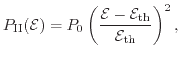
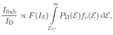
In the work of Rauch and La Rosa [211,212], a compact modeling approach for the total substrate current is presented. Although this compact model cannot be used for TCAD, it highlights the importance of the shape of the distribution function. Here, the substrate current of an n-MOSFET is formulated as
As shown in Fig. 5.6(a) the maximum of the integrand depends on the slope of the carrier energy distribution and results according to (5.25) in
| (5.26) |
 |
(5.27) |
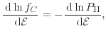
In down-scaled devices the carrier energy distribution exhibits a knee near the
maximum energy available from the steep potential drop along the pinch off
region which is approximated as
![]() [211]. Due to the
constantly rising scattering rate and the abrupt decrease of the carrier
distribution function near the knee point the maximum of the integrand in
(5.23) at
[211]. Due to the
constantly rising scattering rate and the abrupt decrease of the carrier
distribution function near the knee point the maximum of the integrand in
(5.23) at
![]() coincides with the knee near (see
Fig. 5.6(b))
coincides with the knee near (see
Fig. 5.6(b))
In this case the dominant energy is determined by the knee of the distribution function, which by itself depends on the bias conditions and therefore on the available energy [215]. Further influences of voltage changes seam not to shift this peak level. Hence, the final rate is proposed to be
 |
(5.29) |
|
This particular idea of this compact model is to combine the two regimes in one model. It herby highlights the necessity of new modeling paradigms when proceeding to small, down-scaled devices. The validity of both regimes has been shown in [211].
![$\displaystyle \ensuremath{\alpha _\nu}= \ensuremath{\alpha ^{\infty}}_\nu \exp ...
...ft( \frac{\ensuremath{E^{\mathrm{crit}}}_\nu}{E} \right)^{\beta_\nu} \right ] ,$](img358.png)
![\includegraphics[width=0.51\textwidth]{figures/GII200_html.eps}](img397.png)
![\includegraphics[width=0.51\textwidth]{figures/GII50.eps}](img398.png)
![\includegraphics[width=0.48\textwidth]{figures/II.eps}](img399.png)
![\includegraphics[width=0.49\textwidth]{figures/output_II.eps}](img400.png)
![\includegraphics[height=69mm]{figures/ii_rauch_field}](img432.png)
![\includegraphics[height=69mm]{figures/ii_rauch_energy}](img433.png)