4.4.2 High-Field Mobility for DD Equations

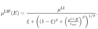
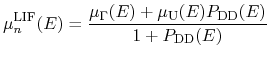
The models proposed for the high-field mobility are based on the mobility expression of the form [352]:

$$\mu^\ensuremath{\mathrm{LIF}}(E)=\frac{\mu^\ensuremath{\mathrm{LI... ...athrm{LI}}\cdot E}{v_\ensuremath{\mathrm{sat}}}\right)^\beta\right)^{1/\beta}}.$$ (4.66)

$\mu^\ensuremath{\mathrm{LI}}$ is the low-field electron mobility as calculated previously, $v_\ensuremath{\mathrm{sat}}$ is the electron saturation velocity, $E$ is the electric field. The same expression was used in [353].

For the DD high-field mobility two different models are available. The first is the convenient model used for Silicon, referred as Model A. The second one is a modified model which can account for negative differential mobility (NDM), referred as Model B. The latter is especially tailored to describe the transport properties of electrons in Nitrides. Further, based on Model B a corresponding HD model can be synthesized.

Model A:

The basic high-field mobility model has the form:

$$\ensuremath{\ensuremath{\mu}_\nu}^\ensuremath{\mathrm{LIF}}\left(... ...\nu}}_\nu}\right)}^{\beta_{\nu}}\right)^{1/\beta_{\nu}}} ,\hspace{5mm} \nu=n,p$$ (4.67)

where $F_\nu$ is the driving force, defined as:

$$F_\ensuremath{\mathrm{n}} = \left\vert \ensuremath{\ensuremath{\ensuremath{\mathitbf{\nabla}}... ...thrm{k}}_\ensuremath{\mathrm{B}}T_\mathrm{L}}{\mathrm{q}} n \right)\right\vert,$$

$$F_\ensuremath{\mathrm{p}} = \left\vert \ensuremath{\ensuremath{\ensuremath{\mathitbf{\nabla}}... ...thrm{k}}_\ensuremath{\mathrm{B}}T_\mathrm{L}}{\mathrm{q}} p \right)\right\vert,$$

for electrons and holes, respectively. The saturation velocity $v_\mathrm{sat,\nu}$ can be calculated in a separate model, accounting for temperature dependence. The parameter $\beta$ models the slope of the mobility increase with increasing electric field, respectively driving force. While in the DD model it can be varied, a corresponding HD model can be obtained only for certain values. Therefore, for electrons in all three materials a value of $\beta$=1 is adopted.

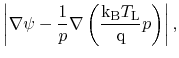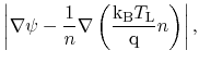
The model is derived from (4.66), with $\xi$=1/2 and using the driving force $F$ instead of the electric field $E$. It offers excellent convergence behavior and a straight-forward calibration method. However, it cannot account for the velocity decrease at higher electric fields. Yet it offers a reasonable agreement with the experimental data and MC simulation results for electric fields below the maximum velocity for all three materials (Fig. 4.16, Fig. 4.17, and Fig. 4.18) using the parameter setup provided in Table 4.8.

Table 4.8: Parameters for DD high-field electron mobility Model A.

	$v_\ensuremath{\mathrm{sat}}$	$\beta$
	[cm/s]	[1]
GaN	3.0$\times$10$^7$	1.0
AlN	3.7$\times$10$^7$	0.45
InN	5.0$\times$10$^7$	1.3

Figure 4.16: GaN electron drift velocity versus electric field: simulations with different mobility models compared to MC simulation results and experimental data.

Figure 4.17: AlN electron drift velocity versus electric field: simulations with different mobility models compared to MC simulation results.

Figure 4.18: InN electron drift velocity versus electric field: simulations with different mobility models compared to MC simulation results.

Model B:

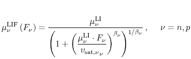
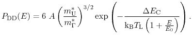
The model is based on the same expression for the mobility (4.66), with $\beta$=1 and $\xi$=1/2. In order to approximate the mobility decay due to intervalley transfer at high fields, two sets of $\mu$ are used. One describes the mobility $\mu_\Gamma(F)$ in the lower valley and the other one in the higher $\mu_\ensuremath{\mathrm{U}}(F)$ (while $\Gamma$ and U are the lowest two valleys only in GaN, this notation is retained for the other materials for simplicity):

$$\mu_\ensuremath{\mathrm{\Gamma}}(E) = \frac{\mu_\ensuremath{\mathrm{\Gamma}}^\ensuremath{\mathrm{LI}}}{... ...a}}^\ensuremath{\mathrm{LI}} E}{v_\ensuremath{\mathrm{sat, \Gamma}}}\right)} ,$$ (4.68)

$$\mu_\ensuremath{\mathrm{U}}(E) = \frac{\mu_\ensuremath{\mathrm{U}}^\ensuremath{\mathrm{LI}}}{1 + \... ...thrm{U}}^\ensuremath{\mathrm{LI}} E}{v_\ensuremath{\mathrm{sat, U}}}\right)} .$$ (4.69)

A weighted mean is built:

$$\ensuremath{\ensuremath{\mu}_{\ensuremath{n}}^{\ensuremath{\mathr... ...c{\mu_{\Gamma}(E)+\mu_{\mathrm{U}}(E) P_{\mathrm{DD}}(E)}{1+P_{\mathrm{DD}}(E)}$$ (4.70)

where $P_{\mathrm{DD}}(F)$ is the valley occupancy [354]:

$$P_{\mathrm{DD}}(E) = 6 A \left(\frac{m_{\mathrm{U}}^*}{m_{\Gamma... ...m{k}}_\ensuremath{\mathrm{B}}T_\mathrm{L} \left(1+\frac{E}{E_0}\right)}\right).$$ (4.71)

$m_{\Gamma}^*$ and $m_{\mathrm{U}}^*$ are the electron masses in the $\Gamma$ and $U$ valleys, respectively, and $\Delta E_\ensuremath{\mathrm{C}}$ is the difference in the conduction bands.

This model allows to set a lower electron mobility and velocity in the higher conduction band. Thus, the characteristic electron velocity decrease of most Nitrides can be described well.

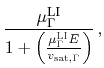
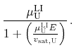
Since all MC simulations and experiments, on which we rely to calibrate the low-field mobility in GaN, were performed at low electric fields, we set $\mu_\Gamma$= $\ensuremath{\ensuremath{\mu}_\nu^{\ensuremath{\mathrm{LI}}}}$ as calculated by the low-field mobility model. Using a down-scaled mobility ( $\mu_\ensuremath{\mathrm{U}}=0.1\times\ensuremath{\ensuremath{\mu}_\nu^{\ensuremath{\mathrm{LI}}}}$ supported by MC data) and velocity in the higher band results in a decrease of the electron velocity at higher fields. With the parameters listed in Table 4.9, the model delivers an acceptable approximation in comparison to MC simulations, accounting for as much as six bands [355] (Fig. 4.16). Results from different groups vary widely (e.g. peak velocity from $2.5\times 10^7$ cm/s to $3.5\times 10^7$ cm/s), therefore our goal is not really a perfect agreement with this particular MC simulation. The model (and the corresponding HD model) is a carefully chosen trade-off. On the one hand they provide a velocity-field characteristics close to the one obtained by MC simulation, while on the other hand they maintain low calculation complexity and a good convergence behavior. An extension accounting for three valleys is possible, however, it was ruled out due to the downgraded convergence of the solution process.

Table 4.9: Parameters for DD high-field electron mobility Model B.

	$v_\ensuremath{\mathrm{sat,\Gamma}}$	$v_\ensuremath{\mathrm{sat,U}}$	$\mu_\Gamma$	$\mu_\ensuremath{\mathrm{U}}$	$\Delta E_\ensuremath{\mathrm{C}}$	$m_{\Gamma}^*/m_0^*$	$m_\ensuremath{\mathrm{U}}^*/m_0^*$	$F_0$
	[cm/s]	[cm/s]	[1]	[1]	[eV]	[1]	[1]	[V/m]
GaN	3$\times$10$^7$	10$^7$	$\mu^\ensuremath{\mathrm{LI}}$	0.1 $\times\mu^\ensuremath{\mathrm{LI}}$	1.4	0.2	0.3	0.26
InN	6$\times$10$^7$	10$^7$	$\mu^\ensuremath{\mathrm{LI}}$	0.1 $\times\mu^\ensuremath{\mathrm{LI}}$	1.78	0.25	0.4	0.035

For AlN, the model cannot be applied due to the very slow increase of the velocity versus electric field. In order to model the latter properly $\beta$=0.45 is needed, however, while being straightforward for the DD model, this will increase considerably the complexity of the corresponding HD model. Therefore, no parameter setup is given here for AlN.

Based on the recent MC simulation studies for InN (accounting for the re-evaluated band gap), a parameter setup is extracted (Table 4.9). Due to the value of $\beta$ close to 1, a good agreement can be achieved (Fig. 4.18) for velocity characteristics below the maximum, while a low value of $F_0$ accounts for the intervalley transfer at fields starting at 50 kV/cm.