


Next: 3.9 Dosis Conservation
Up: 3. Diffusion Phenomena in
Previous: 3.7 Dopant Diffusion in
Subsections
3.8 Numerical Handling of the Diffusion Models
In following section we will present discretization approaches for several diffusion models described in the preceding sections.
Starting with the partial differential equations which model the given diffusion phenomena, we construct the nucleus matrix and residuum vector which are needed to carry out the procedure presented in Section 2.8.
Throughout this section the number of nodes of discretization
 is denoted as
  .
.
3.8.1 Discretization of the Simple Diffusion Model
The discretization of the simple diffusion models follows directly from the discussion presented in Section 2.3. In order to construct the global matrix of the system, we write nucleus matrix of the simple diffusion model for each
 ,
,
 ,
,
 |
(3.76) |
 is the time step of the discretisized time and
 and
and
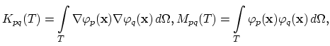
 the stiffness and mass matrices defined on single tetrahedra
  from
,
from
,
for
 . This problem is linear and the calculation of the nucleus matrix
 as the Jacobi matrix of the operator
 (introduced previously in Section 2.5) is trivial.
the global matrix
 is assembled out of the
matrices and has obviosly a dimension equal to the number of all points of discretization.
is assembled out of the
matrices and has obviosly a dimension equal to the number of all points of discretization.
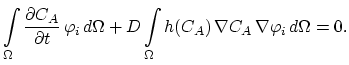
3.8.2 Discretization of the Simple Extrinsic Diffusion Model
We take the functions
 ,
,
 and
and
 defined on
bounded open domen
defined on
bounded open domen  .
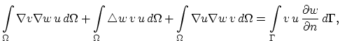
Starting from Green's theorem, a simple relationship can be proved,
.
Starting from Green's theorem, a simple relationship can be proved,
 |
(3.77) |
where  is the boundary of the domain .
We write (3.33) as
is the boundary of the domain .
We write (3.33) as
 |
(3.78) |
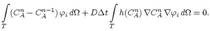
By multiplying (3.78) with the basis function
 and integrating over the domen we have,
 |
(3.79) |
Applying (3.77) on (3.79) gives,
 |
(3.80) |
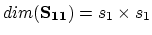
Assuming zero-Neumann boundary conditions on we
obtain the weak formulation of the equation (3.33)
 |
(3.81) |
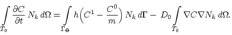
By introducing time discretization with time step and writing the last equation for the single element
we obtain,
 |
(3.82) |
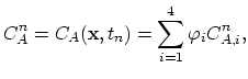
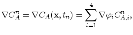
Functions
 ,
,
 , and
, and
 , for
, for
 , are linearly approximated on the element
,
, are linearly approximated on the element
,
 |
(3.83) |
 |
(3.84) |
 |
(3.85) |
The
 , are the values of the concentration at the nodes of the element ,
  is the concentration value at some point inside the .
Normally, for
is the concentration value at some point inside the .
Normally, for
 we use the following simple approximation,
 |
(3.86) |
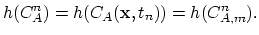
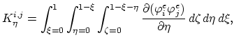
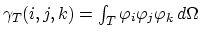
We can define discrete operator  for each
.
Since we have to deal only with a single partial differential equation and not with a system of equations, we can omit the second index in (2.27) by defining the operator,
for each
.
Since we have to deal only with a single partial differential equation and not with a system of equations, we can omit the second index in (2.27) by defining the operator,
 |
(3.87) |
The nucleus matrix is than defined as
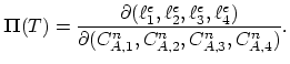 |
(3.88) |
and the residuum vector as,
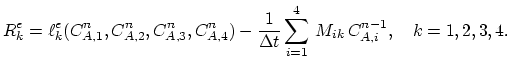 |
(3.89) |
The nucleus matrix for this simple case can be also calculated analytically. In this case is also
 .
.
3.8.3 Discretization of the Three-Stream Mulvaney-Richardson Model
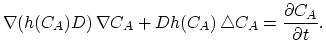
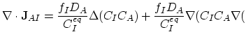
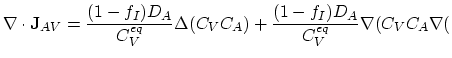
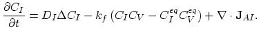
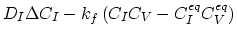
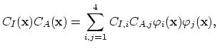
First we consider dopant continuity equation of Mulvaney-Richardson model (3.45).
The local change of dopants is due to the divergence of fluxes of dopant-interstitial and dopand vacancy pairs,
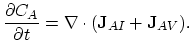 |
(3.90) |
In this model the diffusion coefficient  of the point defect-dopant pairs is considered constant and we can write (based on (3.45)),
 ln ln |
(3.91) |
 ln ln |
(3.92) |
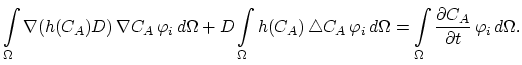
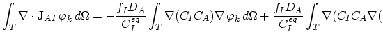
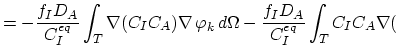
In order to obtain a weak formulation of (3.91) on the single element
we multiply both sides of the equation with the basis function  , and integrate over ,
 ln ln |
(3.93) |
 ln ln |
(3.94) |
The nonlinear terms of (3.94),
 ,
,
 , and
ln
, and
ln are expressed by the basis nodal functions
 on the following way,
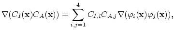 |
(3.95) |
 ln ln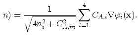 |
|
In the last expression we used the relationship (3.13) for the electron concentration  in the case of single charged dopant.
We substitute the relationships (3.95) into (3.94) and obtain,
in the case of single charged dopant.
We substitute the relationships (3.95) into (3.94) and obtain,
 |
(3.96) |
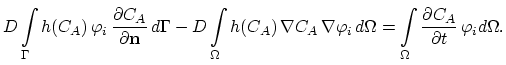
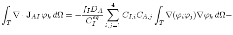
To complete the formulation of the weak equation form we have to evaluate following two integrals,
 |
(3.97) |
 |
(3.98) |
here we transfer the calculation to the normed
 coordinate system. Transformation of the gradient operators is done by multiplication with the matrix
 .
.
 |
(3.99) |
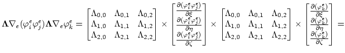
Furthermore we rearrange (3.99),
 |
(3.100) |
and introduce the matrix
 ,
,
 ,
,
 .
.
 |
(3.101) |
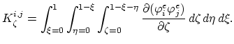
The values of the integrals (3.97) and (3.98) can be expressed as functions of local node indexes,
 |
(3.102) |
 |
(3.103) |
In (3.102) and (3.103), for the sake of simplicity, we used the abbervations,
 for
for
 .
It can easily been shown that the functions
.
It can easily been shown that the functions
 and
and
 satisfy following relations,
 |
(3.104) |
 |
(3.105) |
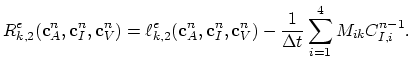
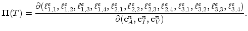
We introduce now the backward Euler time discretization scheme for (3.90) and by applying the functions
 and
and
 we write the
 functions (for
  ),
),
 |
(3.106) |
 |
(3.107) |
and residuum vector  as
as
 |
(3.108) |
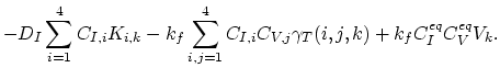
Equations (3.74) and (3.75) of the Mulvaney-Richardson model have the same structure, it is sufficient, if we consider in more detail only (3.74),
 |
(3.109) |
We need to consider only
 , the rest of the equation has already been treated above. Again, we use linear basis nodal functions and apply Green's theorem,
 |
(3.110) |
we set
 , and proceed,
 |
(3.111) |
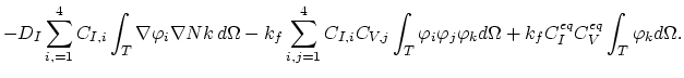
Finally, we have the discretizied form of equation (3.74),
 |
(3.112) |
and the residuum vector  as,
as,
 |
(3.113) |
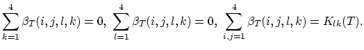
and analogously for the vacancy balance equation,
 |
(3.114) |
and the corresponding residuum vector  as,
as,
 |
(3.115) |
Using the functions
 ,
,
 , and
, and
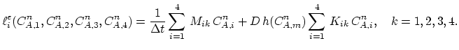
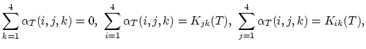
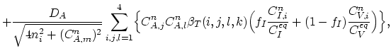
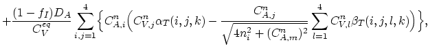
 for we construct the nucleus matrix
of the diffusion problem,
for we construct the nucleus matrix
of the diffusion problem,
 |
(3.116) |
Note that the global matrix
in this case has rank  .
.
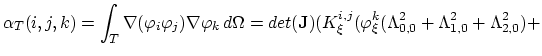
In order to assess the numerical scheme for the problem described in Section 3.5.3 it is useful to construct
an analytical solution for a special one-dimensional case. For the sake of simplicity, we consider in both segments intrinsic diffusion (Section 3.3.1).
As segment  the region
  is assumed and as segment
  region
  .
The one-dimensional segregation problem fullfils the following initial and interface conditions,
.
The one-dimensional segregation problem fullfils the following initial and interface conditions,
 and and |
(3.118) |
 at interface at interface |
(3.119) |
Note that condition (3.117) also means that the media from both sides
of the interface has an infinite length.
We are searching for the solution of the problem given by (3.30), (3.117),
(3.118) and (3.119) in the form,
for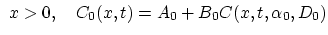 |
(3.120) |
for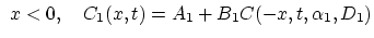 |
(3.121) |
where
 are constants to be
determined and
are constants to be
determined and
is a solution of the diffusion equation (
 ) for the
case of the surface evaporation condition already
studied in [38].
) for the
case of the surface evaporation condition already
studied in [38].
We determine constants
from the initial and interface conditions
(3.117), (3.118), (3.119) as follows.
From the initial conditions we have
 and and |
(3.123) |
The interface condition (3.119) yields
 |
(3.124) |
This equation is fullfiled if
 and and |
(3.125) |
From (3.118) and (3.123) follows,
 erfc erfc |
(3.126) |
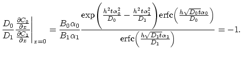
The last equality is ensured for the condition,
 and and |
(3.127) |
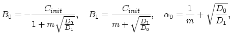
By solving the equation system given by (3.125) and
(3.127) we have,
 |
(3.128) |
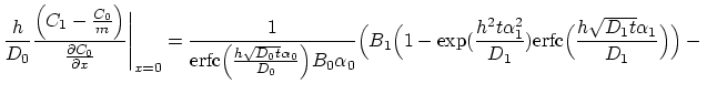
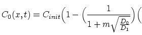
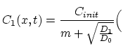
So we can write a solution for the problem posed by (3.30), (3.117),
(3.118) and (3.119). For ,
and for ,
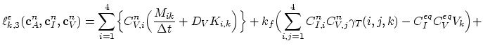
3.8.5 Numerical Handling of the Segregation Model
Let us assume that the segments and are comprised of
three-dimensional areas  and
and  and
the connecting interface
and
the connecting interface  with two-dimensional area
 , respectively. The tetrahedralization of areas ,
and the
triangulation of area are denoted as
, respectively. The tetrahedralization of areas ,
and the
triangulation of area are denoted as
 ,
,
 and
and
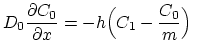
 . We discretize (3.30) on the
element
. We discretize (3.30) on the
element
 using a
linear basis function . After introducing the weak formulation of the equation and subsequently applying Green's theorem we have
using a
linear basis function . After introducing the weak formulation of the equation and subsequently applying Green's theorem we have
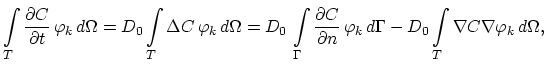 |
(3.131) |
where is the boundary of the element .
Assuming that
 and
marking all inside faces of as
and
marking all inside faces of as
 we have
 and we can write
 |
(3.132) |
In the standard finite element assembling procedure [5], we take into
account only the terms
 when
building up the stiffness matrix. Thereby the terms
when
building up the stiffness matrix. Thereby the terms
 do not need to be considered because of their annihilation on the inside faces.
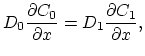
The term
 makes sense only on the interface area and
there it can be used to introduce the influence of
the species flux from the neighboring segment area by applying
the segregation flux formula (3.65)
makes sense only on the interface area and
there it can be used to introduce the influence of
the species flux from the neighboring segment area by applying
the segregation flux formula (3.65)
 |
(3.133) |
After a usual assembling procedure on the tetrahedralization
and
has been carried out and the global
stiffness matrix for both segment areas of the segregation problem has been built,
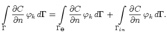
the interface inputs (3.131) for the segregation fluxes  and
and  are evaluated on the triangulation
and
assembled into the global stiffness matrix according to the particular
assembling algorithm developed in this work.
are evaluated on the triangulation
and
assembled into the global stiffness matrix according to the particular
assembling algorithm developed in this work.
The numerical algorithm based on the concept described above is carried out in two steps.
Step 1.
We assemble the general matrix
of the
problem for both segments, i.e., for both diffusion processes. The number
of points in segments and is denoted as  and
and  ,
respectively. The
general matrix has dimensions
,
respectively. The
general matrix has dimensions
 and the
inputs are correspondingly indexed.
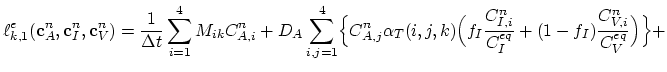
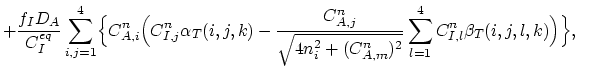
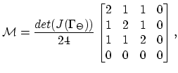
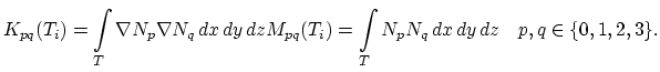
The matrix is assembled by distributing
the inputs from matrix
and the
inputs are correspondingly indexed.
The matrix is assembled by distributing
the inputs from matrix
 ,
,
 , defined for each
 |
(3.134) |
The is the time step
of the discretisized time and
 and
and
 are stiffness and mass matrix defined on single
tetrahedra
are stiffness and mass matrix defined on single
tetrahedra  from
from

Let us denote vertices of the element
from the tetrahedralization
by
 and their indexes in the segment
  by
by
 . Assembling means, for each
 ,
and
,
and
 adding the term
 to
to
 .
.
After this assembling procedure is carried out the general matrix
has the following structure,
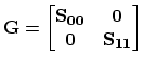 |
(3.135) |
Where
 and
and
 . The matrix
 and
and
 are the finite element discretizations of equation (3.30)
for the segments and , respectively.
are the finite element discretizations of equation (3.30)
for the segments and , respectively.
Step 2.
For the element
 with one of it's faces
(
with one of it's faces
(
 ) laying on the interface according to the idea presented above, weak formulation is,
 |
(3.136) |
The segregation term on the right side of (
 ) is
evaluated on the two-dimensional element
.
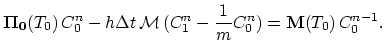
If we discretisize equation (
) is
evaluated on the two-dimensional element
.
If we discretisize equation (
 ) and take a backward Euler time scheme with time step , we obtain for segment ,
 |
(3.137) |
where
 |
(3.138) |
are the values of the species concentration for the  and
and  time step at the vertices of element
  and analogously
 for
for
 ,
,
 .
Without loosing generality we assume that verticex
.
Without loosing generality we assume that verticex  of the tetrahedras and
  is the point which
doesn't belong to the interface .
In that case the matrix
is the point which
doesn't belong to the interface .
In that case the matrix
 from (
 ) has a simple structure,
 |
(3.139) |
where
 is the Jacobi matrix evaluated on element
.
Using (3.132) we have,
is the Jacobi matrix evaluated on element
.
Using (3.132) we have,
 |
(3.140) |
We introduce now
 and
and
 and write for the element ,
 |
(3.141) |
and analogously for the element ,
 |
(3.142) |
In the following, for the sake of simplicity, we omit
from
 and write
 .
.
The contributions of
 and
and
 are already included in the
general matrix
by the assembling procedure
made in the first step, the build up of
can now be completed by adding the inputs from matrix
are already included in the
general matrix
by the assembling procedure
made in the first step, the build up of
can now be completed by adding the inputs from matrix
 and
and
 in order to take into account the segregation effect on interface
.
in order to take into account the segregation effect on interface
.
We denote the vertices of the element
 as
as
 . In the tetrahedralization
these points have indices
. In the tetrahedralization
these points have indices
 and indices
 in the tetrahedralization
.
The actual implementation of the scheme (
in the tetrahedralization
.
The actual implementation of the scheme (
 ) is for each
element
of the interface triangulation
and for
:
) is for each
element
of the interface triangulation
and for
:
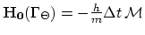
- adding the term
 to the
input
to the
input

- adding the term
 to the
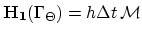
- adding the term
 to
to
- adding the term
 to the
 .
.
Now the assembling of the general matrix
is
completed. These procedure is carried out for each time step of the simulation.
The numerical solution of the segregation problem is compared with an analytical solution on Figure 3.2.
Next: 3.9 Dosis Conservation
Up: 3. Diffusion Phenomena in
Previous: 3.7 Dopant Diffusion in
H. Ceric: Numerical Techniques in Modern TCAD


 erfc
erfc
![\includegraphics[height=0.5\linewidth]{figures/n80m3.eps}](img664.png)
![\includegraphics[height=0.5\linewidth]{figures/n20m0_2.eps}](img665.png)
![\includegraphics[height=0.5\linewidth]{figures/n80m0_2.eps}](img666.png)
 erfc
erfc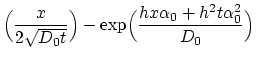 erfc
erfc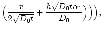
 erfc
erfc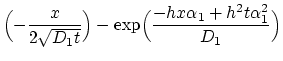 erfc
erfc
![\includegraphics[height=0.5\linewidth]{figures/n20.eps}](img663.png)