In recent years various works on three-dimensional plasma etching simulation have been presented. However, most of them are not suitable to solve complex plasma etching models. The transport equations of more generalized models cannot be solved in three dimensions by the conventional approach, due to computational limitations. For simplification, specular reflections of ions or higher order reemissions of neutrals are often neglected [43,50]. In order to incorporate such effects, particle trajectories must be calculated using the MC technique [64,95]. The ray tracing techniques described in this work derive an efficient solution, even for large three-dimensional structures [A19].
Typical plasma etching models assume ballistic transport of particles at feature-scale and Langmuir-type adsorption [1,14,15,63]. As a representative of these mathematically similar models, the SF![]() /O
/O![]() plasma etching model given in [14] is selected. The surface kinetics model and its governing equations are briefly discussed. However, a more detailed description, including full sets of model parameters, can be found in the original publication [14].
plasma etching model given in [14] is selected. The surface kinetics model and its governing equations are briefly discussed. However, a more detailed description, including full sets of model parameters, can be found in the original publication [14].
The model assumes three different particle species: Fluorine, oxygen, and ions. The arrival directions of neutrals are assumed to follow the cosine law (2.5), while a power cosine distribution (2.8) is used for ions. For the description of the surface kinetics, coverages
![]() and
and
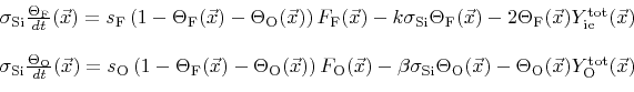
![]() are introduced, which describe the fraction of surface sites covered with fluorine and oxygen, respectively. The corresponding balance equations can be written in analogy to (2.34) as
are introduced, which describe the fraction of surface sites covered with fluorine and oxygen, respectively. The corresponding balance equations can be written in analogy to (2.34) as
 |
(6.1) |
The surface velocity is equal to the total etch rate which is composed of three contributions, chemical etching, physical sputtering, and ion-enhanced etching (2.33)
 |
(6.2) |
The model fully incorporates specular reflexions of ions, which depend on the incident energy and direction. The reemitted direction follows the distribution given in (2.17). The functional dependence of the reemitted energy distribution on the incident energy is described in detail in [15].
The plasma etching process is first applied to a two layer structure, a silicon substrate covered by a
![]() thick SiO
thick SiO![]() mask layer with a circular tapered hole. The diameter of the hole is
mask layer with a circular tapered hole. The diameter of the hole is
![]() at the bottom and
at the bottom and
![]() at the top. The geometry is represented by two LSs resolved on a regular grid with lateral extensions
at the top. The geometry is represented by two LSs resolved on a regular grid with lateral extensions
![]() and a grid spacing of
and a grid spacing of
![]() . Reflective boundary conditions are assumed in both lateral grid directions.
. Reflective boundary conditions are assumed in both lateral grid directions.
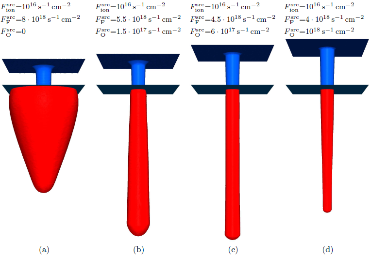
Figure 6.5 shows the LS representations of the profiles after
![]() for different fluxes of oxygen and fluorine from the source. With increasing amount of oxygen, the etched profile gets more directional. The oxygen covers the sidewalls and prevents them from corrosion. Mask etching is also incorporated in these simulations. At every time step 5 million trajectories of each involved particle species are calculated. Due to the spatial subdivision and the use of modern quad-core processors the calculation time of one time step could be reduced to less than
for different fluxes of oxygen and fluorine from the source. With increasing amount of oxygen, the etched profile gets more directional. The oxygen covers the sidewalls and prevents them from corrosion. Mask etching is also incorporated in these simulations. At every time step 5 million trajectories of each involved particle species are calculated. Due to the spatial subdivision and the use of modern quad-core processors the calculation time of one time step could be reduced to less than
![]() . About 2000 time steps are necessary to obtain the final profiles, resulting in a total computation time of approximately
. About 2000 time steps are necessary to obtain the final profiles, resulting in a total computation time of approximately
![]() .
.
 |
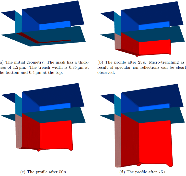
In a further example, a more complex structure (Figure 6.6a) is exposed to the same process parameters as listed in Figure 6.5c. The entire geometry is resolved on a grid with lateral extensions
![]() . Again, reflective boundary conditions and a grid spacing of
. Again, reflective boundary conditions and a grid spacing of
![]() are used. The LS representations of the profile at different times are shown in Figure 6.6. For this simulation, due to the larger domain size, 20 million particle trajectories of each particle species were calculated at every time step. The full incorporation of specular reflections leads to micro-trenching at the trench bottom edges (Figure 6.6b). For the same reason, the bend and the end of the trench are etched deeper.
are used. The LS representations of the profile at different times are shown in Figure 6.6. For this simulation, due to the larger domain size, 20 million particle trajectories of each particle species were calculated at every time step. The full incorporation of specular reflections leads to micro-trenching at the trench bottom edges (Figure 6.6b). For the same reason, the bend and the end of the trench are etched deeper.
 |