3.2.1 Upwind Scheme

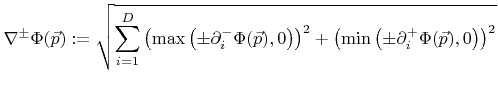
Based on the Engquist-Osher scheme [28], Osher and Sethian proposed a finite difference upwind scheme to solve the LS equation over time [86,110]. The scheme uses the following approximation for the Hamiltonian

$${\hat{H}}({\vec{p}},{\Phi},{V}({\vec{p}})) := \max\left({V}({{\ve... ...hi}({\vec{p}})+ \min\left({V}({{\vec{p}}}),0\right)\nabla^{-}{\Phi}({\vec{p}}).$$ (3.8)

Depending on the sign of the surface velocity ${V}$ this upwind scheme selects an appropriate one-sided approximation for $\lVert\nabla{\Phi}\rVert$

$$\nabla^{\pm}{\Phi}({{\vec{p}}}):=\sqrt{ \sum_{i=1}^{{D}} \left(\m... ...ht)^2+ \left(\min\left(\pm\partial^{+}_{i}{\Phi}({\vec{p}}),0\right)\right)^2 }$$ (3.9)

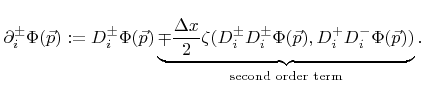
to guarantee a stable solution. $\partial^{\pm}_{i}{\Phi}$ are one-sided approximations to the first derivatives with respect to the $i$ -th direction

$$\partial^{\pm}_{i}{\Phi}({\vec{p}}) := {D}^{\pm}_{i}{\Phi}({\vec{... ...{p}}),{D}^{+}_{i} {D}^{-}_{i} {\Phi}({\vec{p}}) ) }_{\text{second order term}}.$$ (3.10)

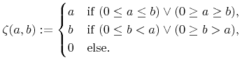
${\zeta}$ is a switch function and is defined as

$${\zeta}(a,b):=\begin{cases}a & \text{if} \ (0\leq a \leq b) \vee ... ... \text{if} \ (0 \leq b < a) \vee (0 \geq b > a),\\ 0 & \text{else.} \end{cases}$$ (3.11)

Depending on whether the second order term in (3.10) is included or not the previous equations describe the second or the first order space scheme as given in [110]. The advantage of these schemes is that they can be straightforwardly implemented without special knowledge of the surface velocity function ${V}$ . However, stability is only guaranteed for convex speed laws. That means the scheme is stable for convex Hamiltonians with respect to the first order derivatives of the LS function $q_i:=\frac{\partial {\Phi}}{\partial{x}_i}$ . This is the case, if the matrix $\left(\frac{\partial^2{H}}{\partial{q_i}\partial{q_j}}\right)$ is positive-semidefinite [110].

Unfortunately non-convex Hamiltonians occur frequently in topography simulations. In the general case the surface velocities depend on the surface normal (see for example (2.24) or (2.36)). As shown later in Section 3.3.1 the surface normal can be expressed using the first order derivatives of the LS function. Hence, the convexity of the Hamiltonian is actually given by the model specific surface velocity function.

Non-convex Hamiltonians occur often, if yield functions are involved, which depend on the incident angle as described by (2.21). Models for anisotropic wet etching processes (see Section 2.3.3) can also lead to non-convex Hamiltonians.