4 Adaptive Visibility Sampling
If the direct flux originating from one or more remote sources above the structure is required to evaluate the surface velocity model, typically either a top-down or a bottom-up approach is used to obtain the flux rates for all points on the surface. The bottom-up approach integrates the flux contribution from the source towards a surface point by
-
• finding all directions that are not obstructed by the geometry, and
-
• integrating the source contribution over these directions,
which yields the surface rates (cf. Section 2.2). The accurate calculation of these surface rates is a significant computational bottleneck in three-dimensional process simulations, especially for high aspect ratios which are increasingly required as device structures move towards full three-dimensional designs, e.g., NAND flash cells [64].
Figure 4.1 conceptually illustrates different stages in one time step of a simulation using a bottom-up integration scheme: (a) A set of integration points is defined on the initial surface. (b) For each integration point, a scheme defines the directions which are tested for direct visibility of the source plane. (c) The surface is advected according to the surface velocity model that requires the results of the integrations (i.e., surface rates).


Figure 4.1: Two-dimensional illustration of a surface advection using a bottom-up integration scheme for direct flux: (a) Initial position of the surface and source plane. (b) Integration points distributed on the initial surface. (c) Integration directions for each integration point. The red directions indicate where the source plane is directly visible. (d) Resulting surface velocities and surface position after the advection.
For an arbitrary geometry, visibility information of the full upper hemisphere (i.e., all upward pointing vertical directions) is required; the lower hemisphere can be neglected as the source plane is always strictly above the surface. The number of required visibility tests depends on the scheme used to define the sampling directions.
The problem to discretize and access data distributed on a sphere is common in many fields [69][65][67][68]. The most straightforward (hemi)spherical tiling is to use a regular grid with respect to the two angular coordinates of a spherical
coordinate system. A disadvantage is that the area of the grid cells decreases towards the poles (i.e., where the polar angle approaches  ), leading to a non-uniform sampling with respect to the subtended solid
angles. Alternative sampling schemes can be derived from subdividing a spherical polyhedron. The platonic solids are a common choice as basis for such tiling schemes [71][72][66]. The concentration of grid cells around the poles is overcome
at the price of irregular coordinates.
), leading to a non-uniform sampling with respect to the subtended solid
angles. Alternative sampling schemes can be derived from subdividing a spherical polyhedron. The platonic solids are a common choice as basis for such tiling schemes [71][72][66]. The concentration of grid cells around the poles is overcome
at the price of irregular coordinates.
In the following, an adaptive sampling scheme to accelerate the direct flux integration during a process simulation is presented [1][2]. It is applicable when a bottom-up approach (cf. Section 2.2) is chosen for the particle transport. An icosahedron, i.e., the platonic solid with the most (=20) faces, and its subdivided versions (to increase the resolution) are used to sample the spherical directions during the numerical integration of the surface rates. The presented scheme reduces the number of rays which have to be traced during the visibility calculation by only refining the sample directions where the visibility changes. The scheme is especially useful for geometric configurations as they occur in Process TCAD, i.e., typically the source plane is visible through one or a few larger apertures. It is shown that if the initial sampling is chosen appropriately, the accuracy of the flux integration is not reduced but the runtime is cut by 50% for higher spatial resolutions.
First, the properties of the hierarchically subdivided icosahedron are presented in more detail. Then, the numerical intgeration scheme of the direct flux is presented. Finally, the adaptive sampling scheme is introduced and results are shown for
a cylindrical hole with aspect ratios  to
to  .
.
4.1 Subdivided Icosahedron
The initial spherical tiling is provided by an icosahedron which consists of 20 equilateral triangles defined by 12 vertices on a spherical surface. To increase the resolution, the triangles are subdivided according to [70]: For each triangle,
-
• compute the midpoints of the edges,
-
• project those midpoints onto the unit sphere,
-
• remove the original triangle, and
-
• connect the three original vertices and the three new midpoints to form four new triangles.
The resulting triangles have similar shape and quality as the original triangles of the icosahedron although they differ slightly in size and are not equilateral.
Figure 4.2 visualizes an icosahedron ( ) and the first four subdivisions (
 to
to  ) together with the integration directions which are defined via the centroids of the triangles.
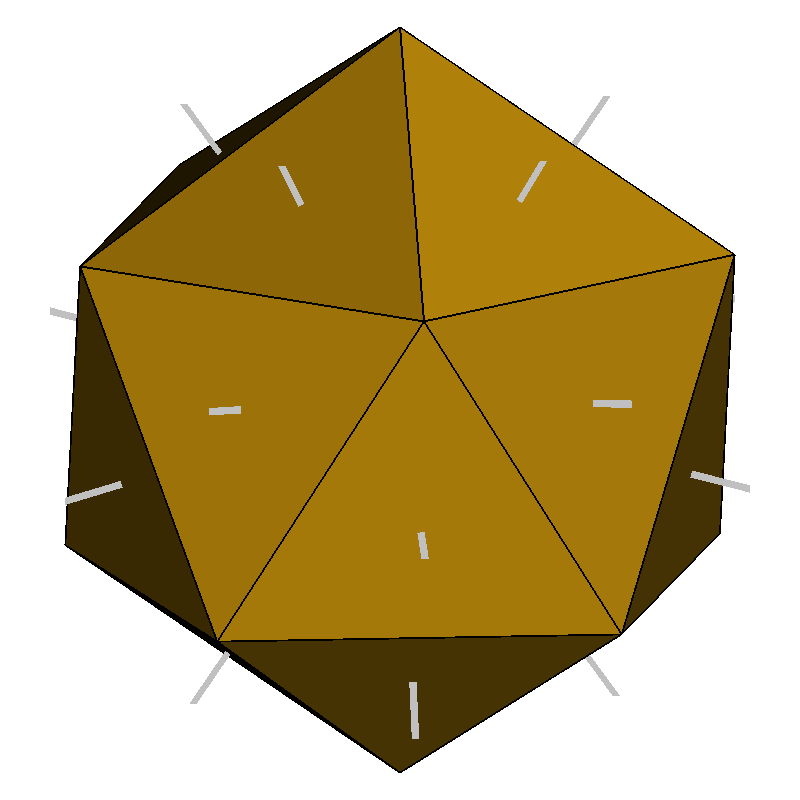
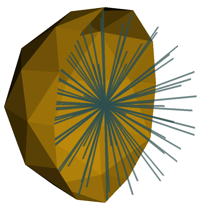

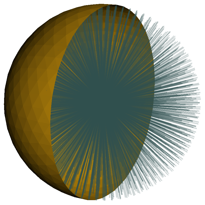
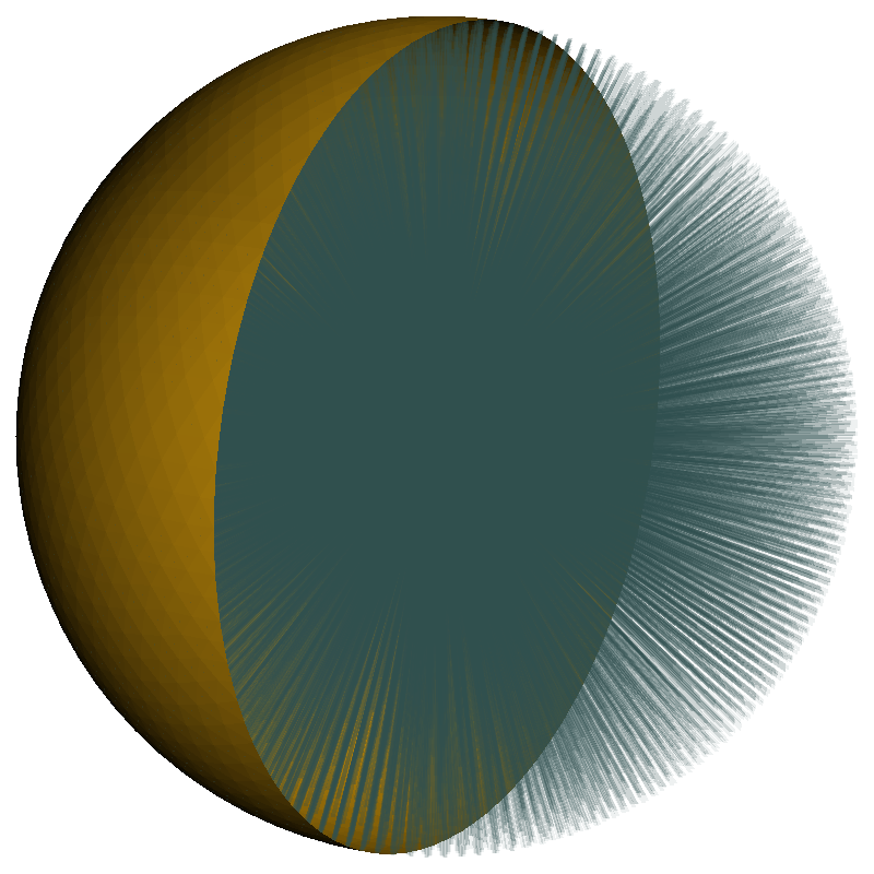
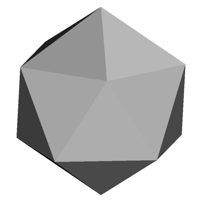
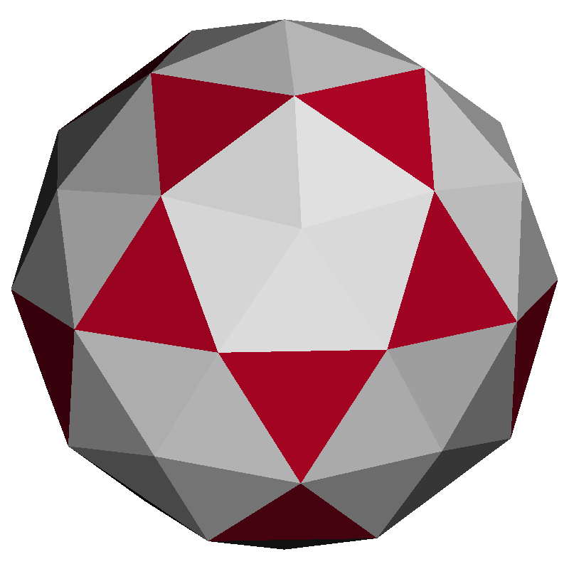
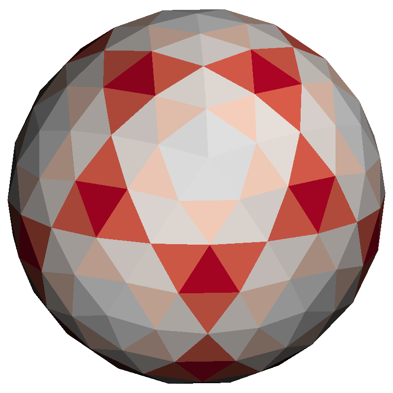
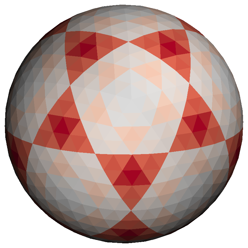
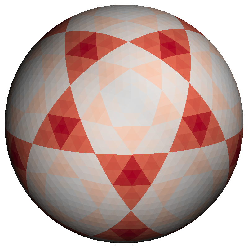
Figure 4.2: Initial icosahedron (n=0) and subdivisions up to n=4. The top row shows the integration directions originating at the center and pointing towards each centroid of the triangles of the spherical mesh. The bottom row visualizes the dif- ferences in the areas of the triangles (gray = smaller, red = larger) resulting from the subdivisions. Detailed numerical information about each subdivision step is listed in Table 4.1.
Table 4.1 provides detailed properties of the original icosahedron and the subdivision steps up to  . The number of triangles for subdivision step
  is defined as

The corresponding number of vertices is defined by

where the first summand originates from the initial vertices shared by five triangles; the subsequent summands originate from the subdivisions which generate vertices shared by six triangles. This difference (i.e., five or six triangles sharing a
vertex) is also the reason for the subdivided triangles not being equilateral and having different areas. The angular resolution  in Table 4.1 is the angle corresponding to a spherical cap of the same area as a triangle. For subdivision step

where an equal distribution of the solid angle over all triangles is assumed. Furthermore, Table 4.1 illustrates the effect of the subdivision on the spread of triangle areas  .
.
| subdivisions |  |
 |
|
|
 |
|||
| n=0 | 20 | 12 | 25.842 | 1.00000 | 0.9000000 | |||
| n=1 | 80 | 42 | 12.839 | 0.84222 | 0.9750000 | |||
| n=2 | 320 | 162 | 6.409 | 0.78820 | 0.9937500 | |||
| n=3 | 1280 | 642 | 3.203 | 0.77377 | 0.9984375 | |||
| n=4 | 5120 | 2562 | 1.602 | 0.77010 | 0.9996094 | |||
| n=5 | 20480 | 10242 | 0.801 | 0.76918 | 0.9999023 | |||
| n=6 | 81920 | 40962 | 0.400 | 0.76895 | 0.9999756 | |||
| n=7 | 327680 | 163842 | 0.200 | 0.76889 | 0.9999939 | |||
| n=8 | 1310720 | 655362 | 0.100 | 0.76888 | 0.9999985 | |||
| n=9 | 5242880 | 2621442 | 0.050 | 0.76888 | 0.9999996 | |||
Table 4.1: Properties of an icosahedron and its subdivisions up to n=9:  number of triangles,
  number of vertices,
  angular resolution,
  ratio of triangle areas,
  smallest radius occurring in triangulation.
The next section presents the numerical integration based on the subdivided icosahedron in more detail.
4.2 Numerical Integration
The integration method permits sources with an arbitrary angular distribution function  with direction
  . The integral of the direct flux

received at surface location  (surface normal =
  ) is approximated by triangulating the hemisphere
  based on a subdivided icosahedron leading to

Here  is the direction towards the centroid of triangle
  and
and  is the area of triangle . A centroid rule (4.6) is used in (4.5) to integrate over the area of a triangle.

Using a visibility function  , which evaluates to
  if a surface is intersected in direction
  , and otherwise, the direct flux at surface location is
![(4.7) \{begin}{align} F_i & = \sum _{j=1}^{N_{tri}} \left [ f_{vis}(\mathbf {\Theta _{c_j}}) \Gamma _{src}(\mathbf {\Theta _{c_j}}) (\mathbf {\Theta _{c_j}} \cdot \mathbf
{n_{i}}) \cdot \Delta _j \right ] \ , \{end}{align}](lateximages/lateximage-478.svg)
where  is the upward pointing normal of the source plane, and is the normal direction of the surface at position .
Validation
A power cosine source distribution with a downward mean direction is used to validate the integration method as it provides analytical solutions for the direct flux received on horizontal and vertical surfaces. The angular distribution functions
are defined as  . For , the angular distribution function is reduced to
  and therefore constitutes an
ideal-diffuse source1 (i.e., a source with a constant particle flux per solid angle and per projected source area). Figure 4.3 visualizes the normalized
angular distribution of a power cosine source from to
and therefore constitutes an
ideal-diffuse source1 (i.e., a source with a constant particle flux per solid angle and per projected source area). Figure 4.3 visualizes the normalized
angular distribution of a power cosine source from to  .
.


Figure 4.4: Direct flux received on a horizontal (a) and vertical (b) surface using the presented integration
method. An unobstructed source with a power cosine distribution with exponents ![\( n=[1,5] \)](lateximages/F3273E6350D5E464283B259E6F9A6795.svg) is used. The resolution of the icosahedron is increased by using up to 5
subdivisions, resulting in a maximal angular resolution
is used. The resolution of the icosahedron is increased by using up to 5
subdivisions, resulting in a maximal angular resolution  degrees (see Table 4.1).
The dotted lines are the analytical solutions obtained from (4.8) and (4.9).
The solid lines in (b) show the average of the flux over all four vertical faces of a cube; the error bars indicate the maximum deviation amongst the four vertical faces.
degrees (see Table 4.1).
The dotted lines are the analytical solutions obtained from (4.8) and (4.9).
The solid lines in (b) show the average of the flux over all four vertical faces of a cube; the error bars indicate the maximum deviation amongst the four vertical faces.
The direct flux originating from an unobstructed power cosine source on a horizontal surface is
![(4.8) \{begin}{align} \label {eq:anal_hori} F_{hori} & = \int _0^{\pi /2}\int _0^{2\pi } \left [ \cos (\theta )^{n+1}\right ] sin \theta d\theta d\varphi = \frac {2}{n+2}\ \pi
\{end}{align}](lateximages/lateximage-491.svg)
and for a vertical surface under the same source
![(4.9) \{begin}{align} \label {eq:anal_vert} F_{vert} & = \int _0^{\pi /2}\int _0^{\pi } \left [ \cos (\theta )^n sin(\theta )sin(\varphi )\right ] sin \theta d\theta d\varphi = 2
\int _0^{\pi /2} \left [ \cos (\theta )^n sin(\theta ) \right ] sin \theta d\theta \ . \{end}{align}](lateximages/lateximage-492.svg)
The derivations of the analytical formulations are provided in Appendix B.1.
In Figure 4.4, the numerical results are compared to the analytical solutions for sources with power cosine exponents and subdivisions up to 5. The flux rates approach the analytical solutions with a relative error below 1% for 3 subdivisions and far below 0.1% for 5 subdivisions.
1 Ideal-diffuse sources are used in Process TCAD to model neutral particles.
4.3 Adaptive Sampling Scheme
For each subdivision level of the icosahedron, the search directions are defined towards the centroids of the triangles of the icosahedron. The subdivision divides each triangle into four triangles on the next level, which cover the same area when projected onto the unit sphere (cf. Figure 4.2). Instead of evaluating all directions on the final subdivision level (maxlevel), the presented adaptive scheme starts on a lower subdivision level (minlevel). After evaluating all directions on minlevel, the boundary of the aperture is identified and all directions in the neighborhood of the boundary are re-evaluated on the next level. The aperture boundary is defined as all triangles which are connected to a vertex which shares triangles with mixed visibility information (cf. blue points in Figure 4.5). This procedure is repeated until maxlevel is reached. The adaptive sampling scheme is conceptually illustrated for two dimensions in Figure 4.5.

Figure 4.5: Two-dimensional illustration of the bottom-up visibility scheme for direct flux calculation for two surface points. The search directions are colored according to the source visibility (red = visible, black = obscured). In three dimensions, the search directions are towards the centers of the triangles of the icosahedron. The green solid angles indicate the neighborhood of the aperture boundary. The blue points are identified as aperture boundary points which are used to define the regions for re-evaluation on the next level. The green arrows indicate the refined search directions near the aperture boundary.
After the detection of the visible directions using the adaptive visibility scheme, the integration is performed with the resolution of maxlevel to provide the same integration accuracy compared to the non-adaptive sampling on maxlevel.
Algorithm 1 describes the adaptive visibility sampling for an integration point on the surface including the integration on the maximum refinement level.
Input: minlevel, maxlevel
Output: flux at surface point
for n = minlevel to maxlevel do
if  then
then
set all directions to be active on level n;
set all visibility information to false level on n;
foreach direction  on level n do
if is active then
trace ray into direction of d;
if ray hit source then set visibility for to true;
if ray hit surface then set visibility for to false;
if n  maxlevel then
foreach direction on level  do
do
set visibility for according to parent on level n
foreach vertex v on level n do
if v is boundary vertex then
foreach triangle t connected to v do
mark all children of t active on next level
if n  maxlevel then
foreach direction on level do
if visibility of direction is true then
integrate flux contribution (cf. (4.5));
add contribution to surface point ;
Algorithm 1: Bottom-up direct flux calculation at surface position using the proposed adaptive visibility scheme and integration on the maximum refinement level.
4.4 Evaluation Results
The algorithm is evaluated using a cylindrical hole with aspect ratios between 1 and 25 and resolutions (i.e., number of level-set grid cells) between  and
and  in the lateral directions (Figure 4.6a). This results in vertical resolutions of up to 1100, which represents computationally challenging evaluation cases. To investigate the sensitivity of the approach towards
geometrical variations, the radius at the bottom is varied by
in the lateral directions (Figure 4.6a). This results in vertical resolutions of up to 1100, which represents computationally challenging evaluation cases. To investigate the sensitivity of the approach towards
geometrical variations, the radius at the bottom is varied by  %, leading to extended and tapered holes (Figure 4.6b).


The choice for the minlevel depends on the aspect ratio of the geometry and is illustrated in Figure 4.7: For a vertical geometry, the minimum angular resolution
required to detect the opening aperture is shown and put in relation to the required number of subdivisions of the icosahedron. The maxlevel is set to 6 for all simulations, which corresponds to about  search directions per hemisphere. This choice allows at least one level of refinement for all tested
aspect ratios between 1 and 25 (cf. Figure 4.7, dotted vertical lines).
search directions per hemisphere. This choice allows at least one level of refinement for all tested
aspect ratios between 1 and 25 (cf. Figure 4.7, dotted vertical lines).

All results were produced using a highly, vertically focused2 ( ) power cosine source distribution
  (cf. Figure 4.3). To verify that the accuracy of the integral indeed does not suffer, the flux rates are compared at various depths of the structure: The flux rates are identical when
applying the proposed algorithm.
(cf. Figure 4.3). To verify that the accuracy of the integral indeed does not suffer, the flux rates are compared at various depths of the structure: The flux rates are identical when
applying the proposed algorithm.
Figure 4.8 shows the cross section of a validation simulation with a linear surface velocity model  for the tapered structure (aspect ratio 6). In Figure 4.8a, the impact of a low maximum level of refinement is demonstrated: The position of the top surface is very inaccurate; this is due to the high derivatives of the source distribution
(i.e., a very directed source) in conjunction with a low spatial sampling during the integration. The aperture is detected but the position of the bottom of the structure varies considerably due to an insufficient sampling of the aperture. In
Figure 4.8b, using maxlevel = 5, the positions at the bottom are symmetric and close to the reference in Figure 4.8c. The position of the top surface still shows a noticeable difference to the analytical solution. In Figure 4.8c, also the top surface is very close to the analytical solution.
for the tapered structure (aspect ratio 6). In Figure 4.8a, the impact of a low maximum level of refinement is demonstrated: The position of the top surface is very inaccurate; this is due to the high derivatives of the source distribution
(i.e., a very directed source) in conjunction with a low spatial sampling during the integration. The aperture is detected but the position of the bottom of the structure varies considerably due to an insufficient sampling of the aperture. In
Figure 4.8b, using maxlevel = 5, the positions at the bottom are symmetric and close to the reference in Figure 4.8c. The position of the top surface still shows a noticeable difference to the analytical solution. In Figure 4.8c, also the top surface is very close to the analytical solution.


Figure 4.8: Cross section of three-dimensional simulation results for a linear surface model  and for the tapered structure of aspect ratio 6 from
  to
to  for different refinement settings (a,b,c). The straight, horizontal lines in the upper part (highlighted by red
circles) indicate the analytical solution for a horizontal surface.
for different refinement settings (a,b,c). The straight, horizontal lines in the upper part (highlighted by red
circles) indicate the analytical solution for a horizontal surface.
2 Highly vertically focused power cosine sources are used in Process TCAD to model vertically accelerated particles (ions).
4.5 Performance Results
The average runtime for the parallelized (OpenMP) direct flux calculation (i.e., runtime consumed by SurfaceratesIF.calcSurfRates(), cf. Section 3.2) was tracked for various combinations of aspect ratios, spatial resolutions, and refinement levels. All performance measurements were performed on WS1. The obtained speedups when applying the presented adaptive sampling algorithm are summarized in Figure 4.9; the corresponding ratio of necessary visibility tests between the non-adaptive and the adaptive simulations are summarized in Figure 4.10.
If the visibility tests constituted the entire computational load and no overhead were introduced to maintain and access the visibility information on different subdivision levels of the icosahedron, the speedup would be expected to match the reduction ratio. Figure 4.9 and 4.10 reveal a factor between the speedup and the reduction: For one level of refinement, the factor is about 2 for all configurations; for 2 and 3 levels of refinement, the factor increases up to 4. The underlying reasons are the overhead of creating and accessing the visibility information (which increases with the number of refinement levels) and the computational load of the integration itself, which is performed on the maxlevel for the full aperture regions.
In summary, when only considering one level of refinement, a minimum speedup of 1.5 is obtained for aspect ratio 1. For surface meshes with more than  triangles (aspect ratios 15 and 25), the speedup is larger than 2 for all configurations.


Figure 4.10: Ratios of necessary visibility tests for the full sampling on maxlevel and the adaptive sampling scheme (configurations identical to Figure 4.9).
4.6 Summary
It is shown that the bottom-up adaptive visibility sampling scheme is able to sustain the accuracy of the direct flux integrals while reducing the integration time by 50% for larger meshes ( triangles), as long as all opening apertures are captured by
the minimum level of refinement.
triangles), as long as all opening apertures are captured by
the minimum level of refinement.
When using more than one level of refinement, the ratio between integration time and ray tracing time limits the obtainable speedup, as the integration is always performed on the maximum level of refinement.