3 Simulation Platform
The platform introduced in this chapter is used as a development platform for implementing and evaluating novel computationally efficient approaches to calculate the particle transport in three-dimensional etching and deposition simulations. The approaches presented in Chapters 4, 5, and 6 were implemented and validated using this platform.
The performance of a particle transport calculation can be investigated detached from a simulation of a dynamic surface, i.e., using
-
• a set of surface geometries with corresponding surface models,
-
• information about the domain and boundary conditions, and
-
• information about the properties of the particle sources.
However, there is a disadvantage when using such a static setup: The accumulated effect of the particle transport method on the final topography at the end of the simulation cannot be assessed as the surface is not advected.
The alternative is to embed the evaluation directly into a process simulator. This provides access to all simulation results and allows for the evaluation of particle transport methods throughout the course of a full simulation. However, most available process simulators (cf. Section 2.1) are closed-source projects and therefore unsuitable. At the time of writing, ViennaTS [87] is the only available three-dimensional fully open-source process simulator. Due to a lack of functionality in ViennaTS regarding geometry construction, serialization of the level-sets, and surface extraction a standalone evaluation platform is desired.
To provide an overview, Figure 3.1 illustrates the sequence of computational tasks during a process simulation using such a simulation platform: First, the domain and the layers (i.e., the level-set functions which delimit the material regions) are created (left column). Then, the main computational tasks in each time step of the simulation (middle column) are
-
• the extraction of an explicit representation of the top layer1, i.e., a triangle mesh including the information of the active material for each triangle,
-
• the calculation of the surface rates for each point on the top layer, which requires the calculation of the particle transport,
-
• the calculation of the surface velocities, i.e., the velocity for each point of the top layer,
-
• the extension of the surface velocities, i.e., preparing a velocity field for all level-set grid points in the narrow band of the top layer, and
-
• the advection of the top layer according to the surface velocity field including an appropriate update of the other layers (cf. Section 3.1).
Finally, the resulting layers and material regions are extracted and saved (right column).

Figure 3.1: Coarse-grained flow chart of the process simulation identifying the main computational tasks: Surface extraction, surface rate calculation, surface velocity calculation, creating of the surface velocity field, and the advection of the layers. The relation of the computational tasks encapsulated by the interface classes (cf. Section 3.2) is indicated.
To minimize development effort, open-source third-party libraries were employed. Briefly, the simulation platform is based on OpenVDB [95], using its sparse volume data structure; the tools provided by OpenVDB to manipulate the sparse data (e.g., narrow band level-set methods for advecting/normalizing level-sets and extraction of explicit surfaces) are also utilized. The ray-surface intersection queries for the calculation of the particle transport are performed using Embree [89] as external ray tracing library. Other ray tracing libraries (cf. Chapter 5) were used for validation and performance evaluations.
In the following, first, the necessary extensions to match the requirements of a feature-scale process simulation are discussed in detail. Then, an overview of the software architecture is given by focusing on the abstract interface classes which decouple the individual computational tasks. Finally, test cases and benchmarks are presented.
1 See Section 3.1 for the definition of top layer.
3.1 Requirements for Feature-Scale Process Simulation
The sparse volume data structure provided by OpenVDB [95] is used for surface representation. In [51] a detailed overview of the hierarchical data structure and implemented algorithms is provided and performance benchmarks are presented. OpenVDB suits the requirements for a level-set-based feature-scale process simulator to large extends as it provides [51]
-
• a configurable sparse data structure for volumetric data with cache efficient sequential access and fast random access (which is used to store the layers),
-
• a multi-threaded narrow band level-set method using TVD-RK explicit time integration schemes and a Godunov scheme combined with WENO schemes for spatial derivatives (which is used for the advection of the top layer),
-
• multi-threaded flow-based re-normalization of the narrow band using the same discretization schemes as for the advection (which is used for normalization of the top layer after each advection),
-
• geometry construction and multi-threaded CSG operations (which are used to update the other layers after the top layer is advected (cf. Section 3.1) and to construct the initial geometries),
-
• ray marching (i.e., ray casting) using the hierarchical volume data structure directly (which is used as a baseline for volume/implicit ray tracing performance, cf. Section 5.2),
-
• a fast dual method for the extraction of quad/triangle meshes (which is used for the extraction of a triangle mesh from the top layer, cf. Section 5.2),
-
• a conversion from quad/triangle meshes to volumes/level-sets (which is used to import explicit geometries), and
-
• serialization/deserialization of volumes/level-sets using a memory efficient file format (which is used to store intermediate and final results of the layers and regions).
Nevertheless, OpenVDB also lacks some requirements for a feature-scale process simulator, namely
-
• a confined domain size with prescribed boundary conditions (which is necessary when simulating only a small region of the wafer surface),
-
• a multi-material level-set advection logic (which is necessary if more than one material region is present in the simulation domain),
-
• a method for surface velocity extension (which is necessary as the surface velocities in a process simulation are only available for the surface, cf. Section 2.3), and
-
• a ray-surface intersection test which considers the confined domain and its boundary conditions.
In the following, the necessary extensions are briefly introduced.
Boundary Conditions
In feature-scale process simulations only a small region of the wafer surface is considered. Therefore, it is necessary to define boundary conditions for the vertical and lateral boundaries of the domain. The spatial position of the vertical
boundary is adopted after each time step according to the new maximum vertical extents of the top layer. Two types of domain boundaries are commonly used for the lateral boundaries in a Process TCAD simulation: Periodic and
reflective boundary conditions. Figure 3.2 illustrates the effect of periodic boundaries  (right) and reflective boundaries
  (left) in two dimensions.

Figure 3.2: Two-dimensional illustration of a simulation domain with a reflective boundary condition on the left side and a periodic boundary condition on the right side. The vertical domain boundaries are infinite, i.e.,
are adopted according to the maximum extents of the top layer surface  (blue); the source plane
  (green) is positioned according to the upper vertical domain extent.
Reflective boundary conditions are possible for all geometries; periodic boundary conditions require that the initial geometry on one boundary matches the geometry on the opposing boundary for each applied dimension in which the boundary condition is applied.
If reflective boundary conditions are used, the emission of the particle sources must be rotationally symmetric with respect to the vertical axis; for periodic boundary conditions, the particle sources do not have this constraint.
The boundary conditions are implemented using a straightforward ghost region approach: The lateral boundaries of the simulation domain are extended by a thin layer of grid cells which are initialized according to the applied boundary condition. The surface advection is performed also for the ghost regions. The values in the ghost regions are discarded and re-initialized after each time step of the simulation. Figure 3.3 illustrates the top layer and ghost regions (blue) for a three-dimensional structure before and after a tilted directional etching (i.e., a non-symmetric particle source).
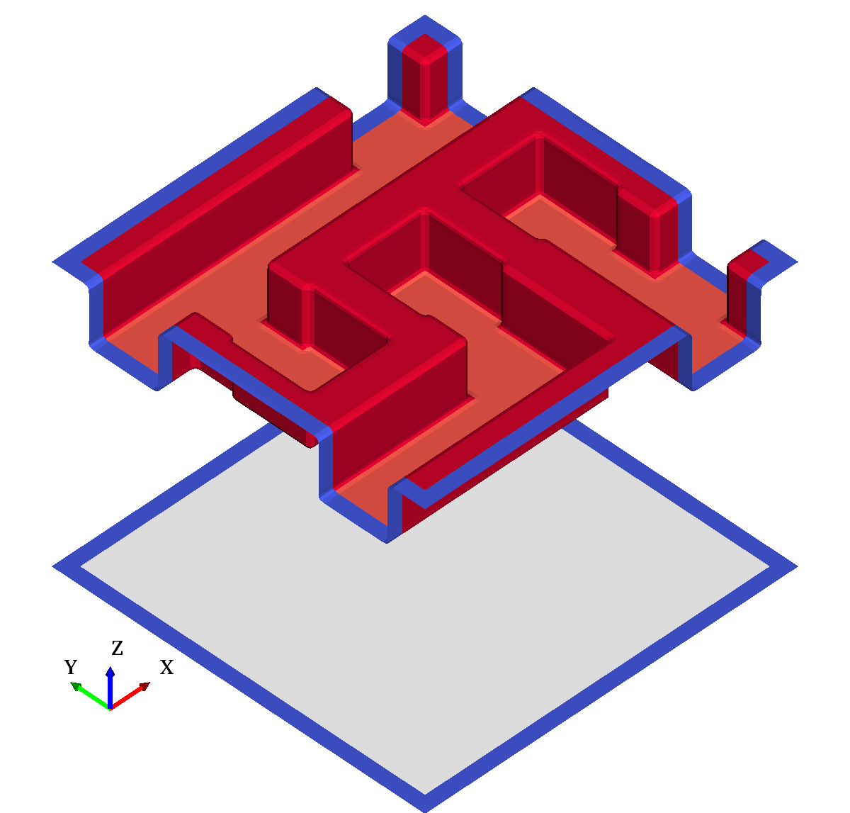
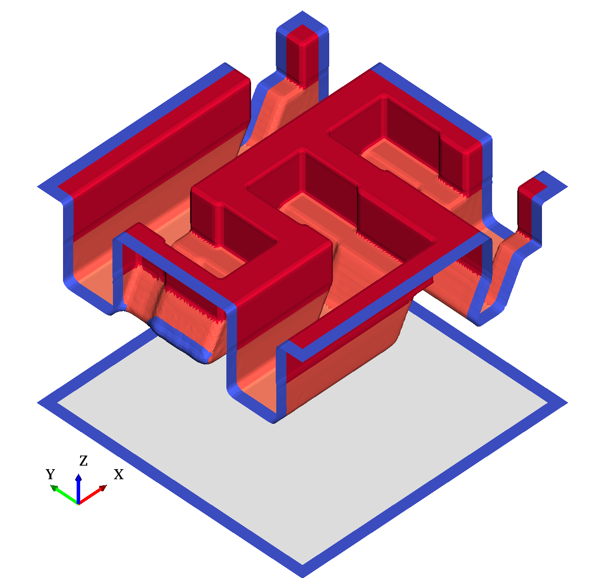
Figure 3.3: Top layer and ghost region of multi-material unidirectional tilted etching test case with periodic boundary conditions. (a) Top layer of
initial geometry where the color indicates the active material and blue is the ghost region. (b) Resulting top layer and ghost region for unidirectional etching
in direction ![\( [-0.5,0,-1] \)](lateximages/B83BD4CEB9BFB64130A943C6A595C623.svg) .
.
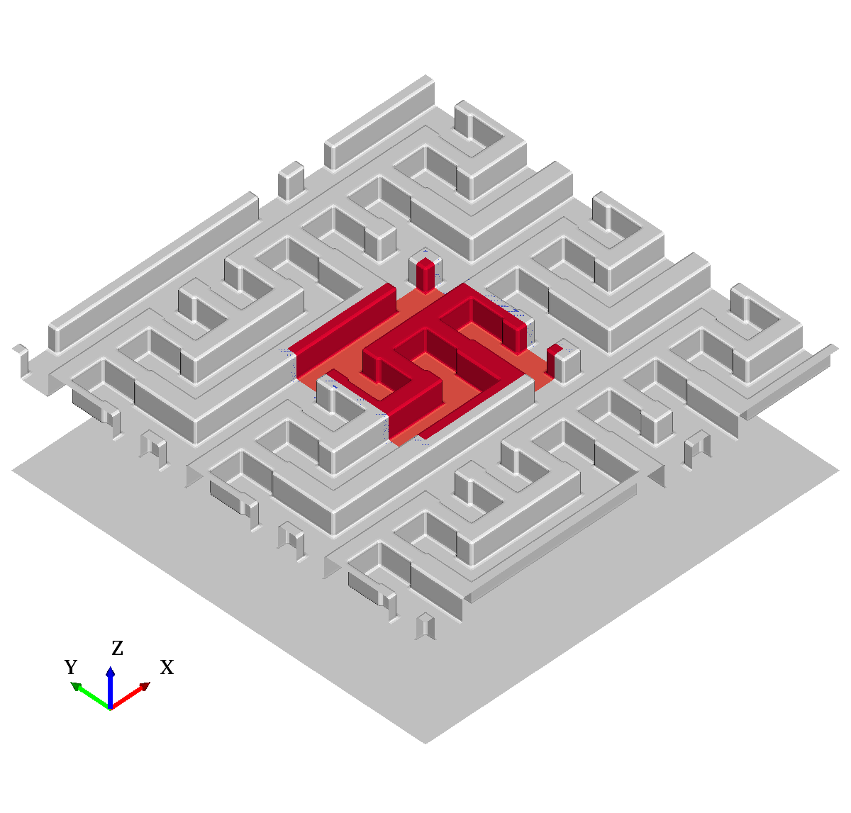
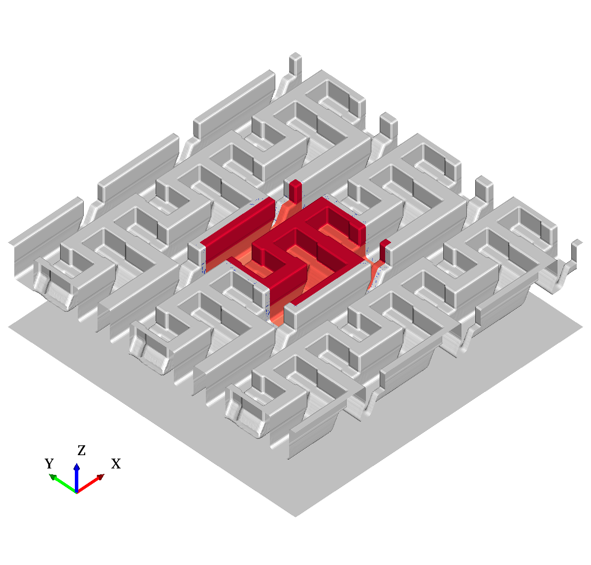
Figure 3.4a illustrates the effective surrounding geometry for the initial geometry of Figure 3.3a, if periodic and reflective boundary conditions are combined. Figure 3.4b illustrates the same simulation results as Figure 3.3b but with the effective surrounding geometry which is produced by the periodic boundary conditions.
Multi-Material Advection
Typically, different material regions are present during an etching process simulation, e.g., a substrate patterned with a mask. Also for deposition processes at least two materials are present, i.e., the initial material and the material which is deposited. The straightforward approach is to represent each material region with a corresponding level-set function. To simultaneously advect all material regions, each region would then be advected separately, leading to potentially mutual penetration. In this case, the parts of a region which are penetrated by another region would be treated inactive, i.e., not subject to advection. One approach would be to perform a Boolean operations between material regions to dissolve the penetrations; in this case a strategy to decide which material fills the former penetrated volume has to be set up.
Another approach [22][87] is to not advect each material region separately but to construct a total union of all regions and advect this top layer. To be able to advect the top layer with the correct surface speed of the
underlying material region, it is necessary to detect the active material for each point on the top layer. This active material for a point  on the top layer is obtained by querying the value of all level-sets at : The construction of the top layer implies that the values of the queries are all
  . The material of the level-set with the smallest value is considered active;
the active material at a point on the surface is therefore
. The material of the level-set with the smallest value is considered active;
the active material at a point on the surface is therefore

where  is the number of materials and
  is the level-set function corresponding to material
  . Additionally, the level-sets have a fixed order and the lower level-set is chosen as active material, if the values
are numerically identical.
. Additionally, the level-sets have a fixed order and the lower level-set is chosen as active material, if the values
are numerically identical.
However, with this approach it is not straightforward to deposit (i.e., the surface velocity  ) multiple materials simultaneously; instead one is restricted to deposit
only one “top material” where . If
) multiple materials simultaneously; instead one is restricted to deposit
only one “top material” where . If  , i.e., material is removed, the top layer is advected according to
the underlying active material. In a subsequent Boolean operation between the advected top layer and each material region, the removal of the material is transferred to the level-sets which represent the materials. The Boolean operation to
subtract the volume penetrated by level-set
, i.e., material is removed, the top layer is advected according to
the underlying active material. In a subsequent Boolean operation between the advected top layer and each material region, the removal of the material is transferred to the level-sets which represent the materials. The Boolean operation to
subtract the volume penetrated by level-set  from level-set
  is
is

A significant advantage of this “top layer” approach is that material layers can be represented with sub-grid resolution. This is possible if the level-sets representing the materials are chosen to not map directly to the material regions, but are constructed “additively”. An example of a three materials setup (illustrated in Figure 3.5a) is used for demonstration: A thick bottom region (blue) is covered by a thin layer (green) which is exposed only in a circular region due to a mask (red). The level-set resolution is chosen such that only a single level-set grid point falls within the vertical span of the green layer.
Figure 3.5b shows a cross section of the (narrow band) level-set grid of the domain. The colored lines mark the extracted zero-level-sets of the regions if the level-sets directly represent the material regions. Figure 3.5c illustrates the same cross section but showing the zero-level-sets, if the level-sets are constructed additively using

where the unions are constructed using

Figure 3.5d once more illustrates the zero-level-sets from Figure 3.5c and additionally shows the reconstructed material regions obtained from

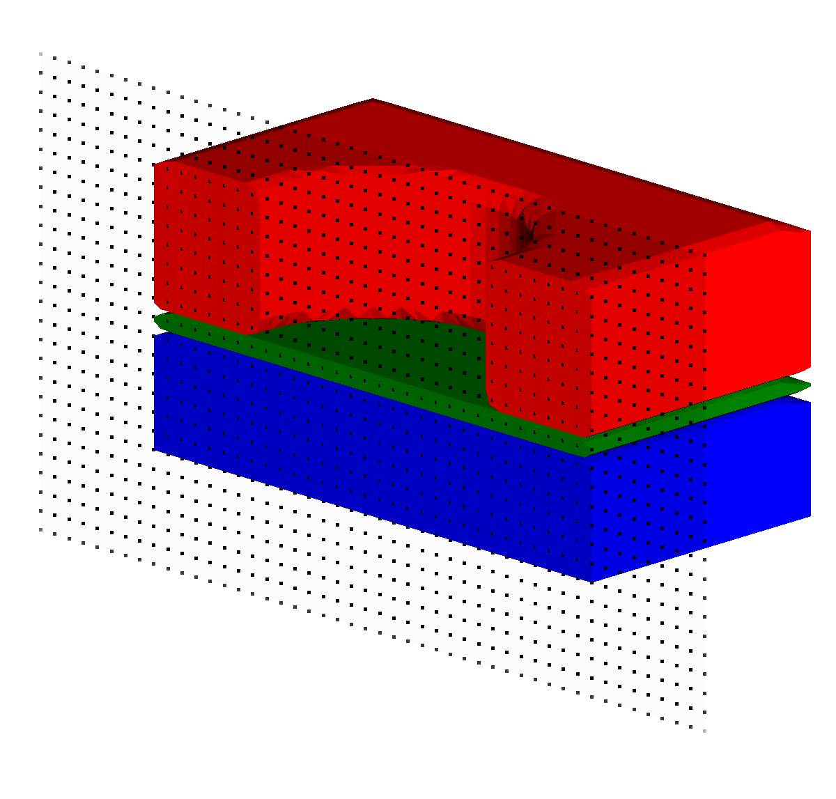
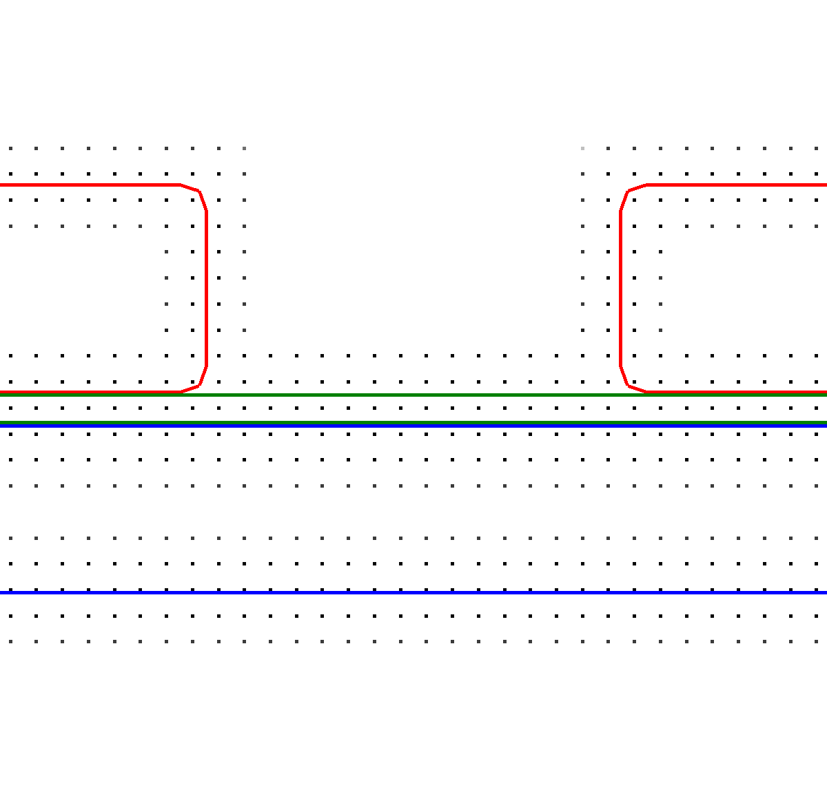
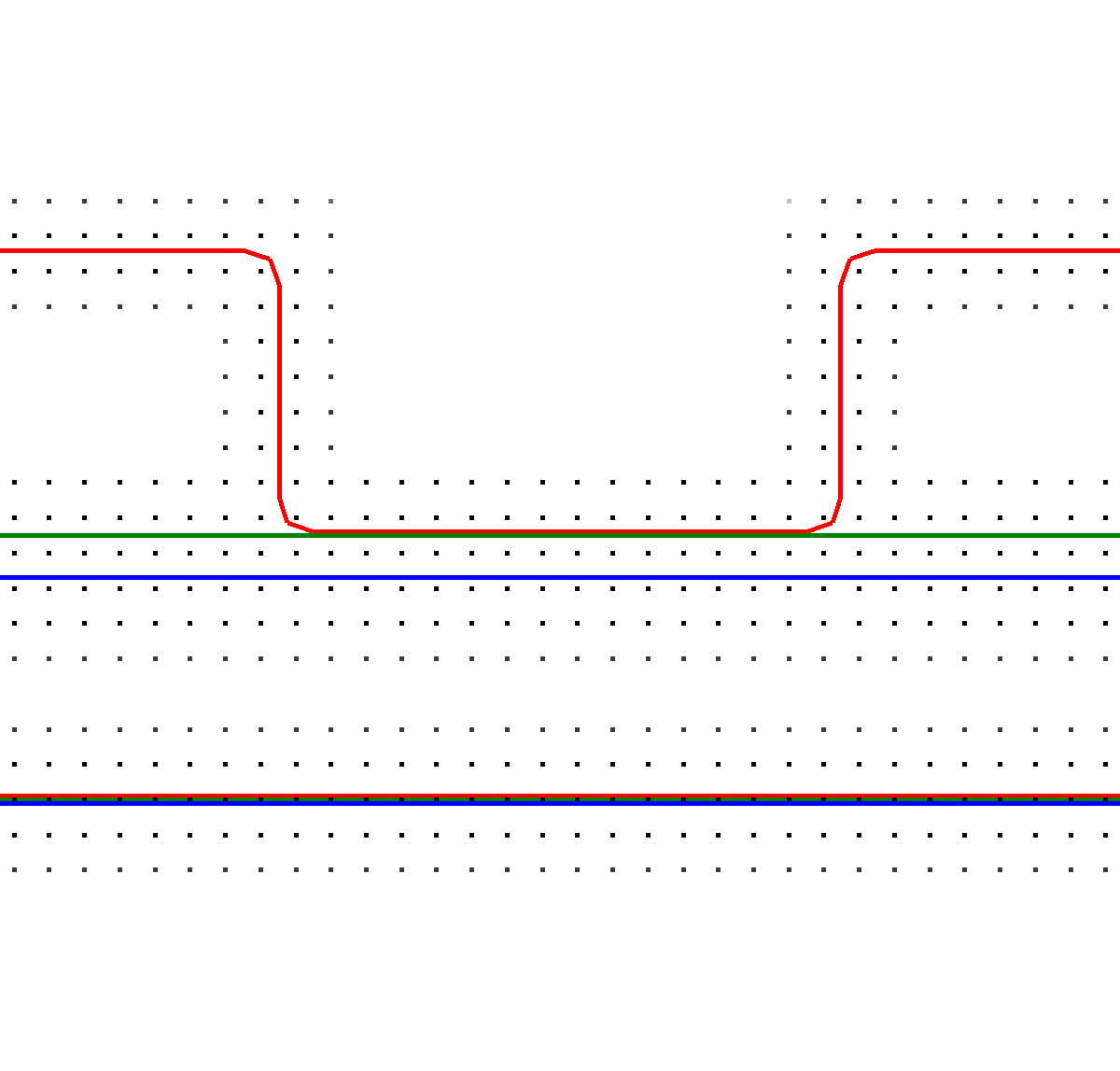
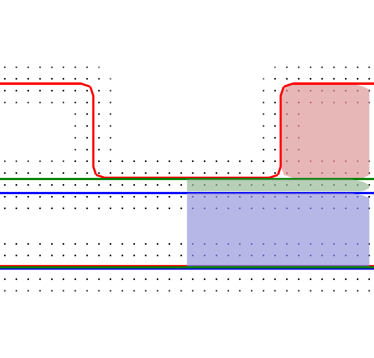
Figure 3.5: Three materials stack with thick bottom region (blue), a thin layer (green), and a mask (red). (a) Cross section through the domain and indicated level-set resolution for the cross section plane. (b) Front view on the right half of the cross section showing the narrow band level-set grid points and the extracted zero-level-sets of the material regions. (c) Representation using an additive scheme from bottom to top in order blue, green, and red. (d) Material regions reconstructed from the level-set of the additive scheme.
Figure 3.6 chronologically illustrates the development of the material stack using top layer advection and the additive scheme to represent the materials. Starting from Figure 3.6b the green layer is represented with sub-grid resolution, until it is fully etched away in Figure 3.6c. Using a straightforward scheme, the thin region of the green layer cannot be represented from Figure 3.6b onwards. It also becomes apparent that a void is formed between the green and the blue layer already in Figure 3.6a; this is due to the nature of the level-set function which is a scalar field and does not hold directional information.
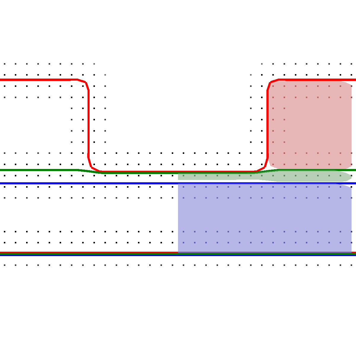

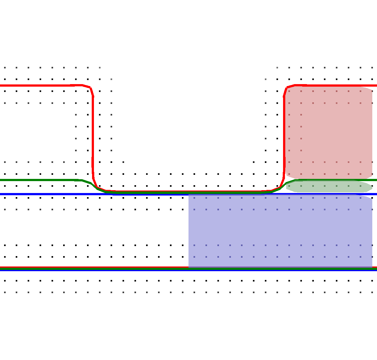
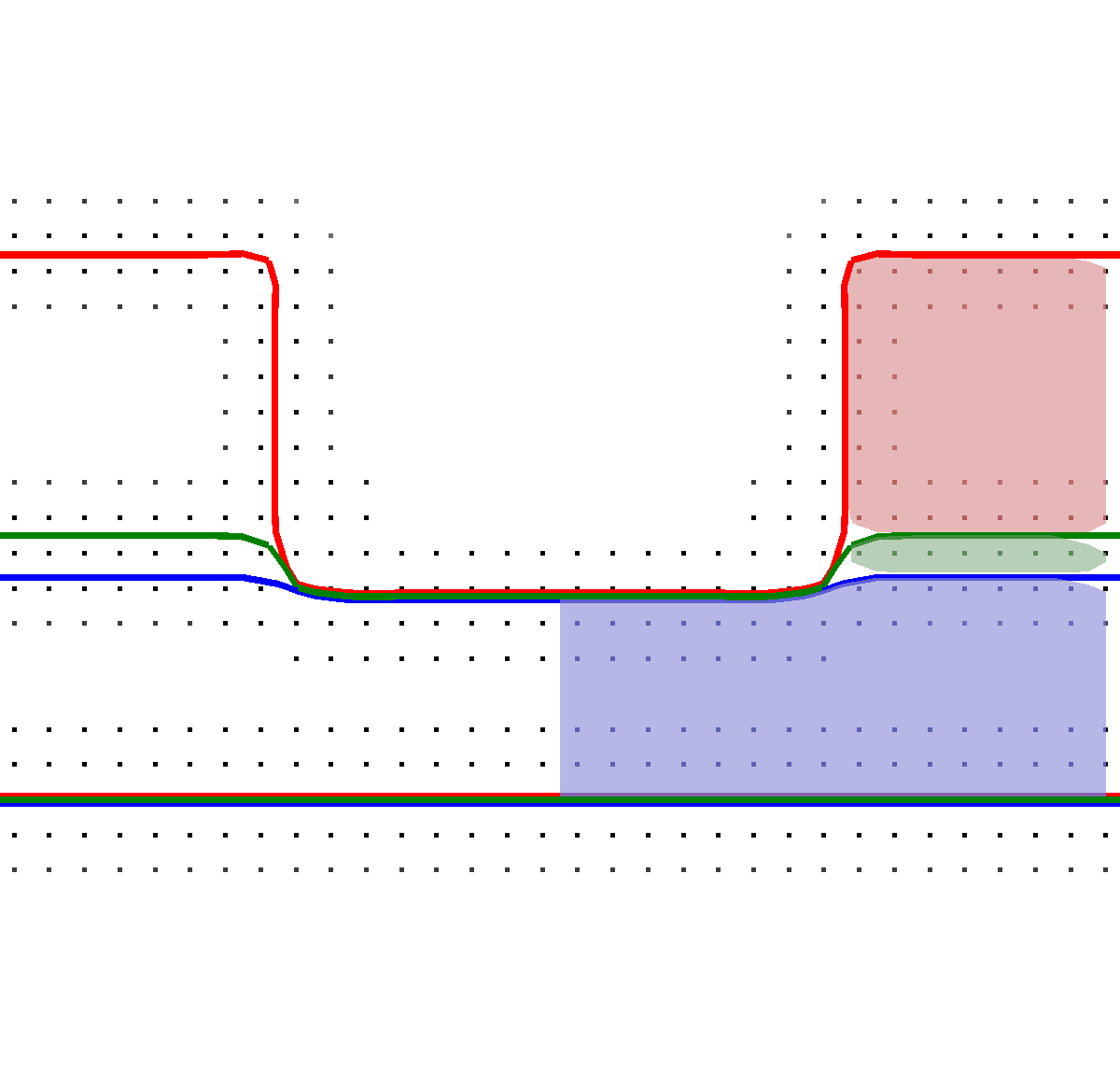
Figure 3.6: Development of the material stack from Figure 3.5 during an isotropic etching simulation using the additive scheme. The zero-level-sets of the additive scheme are shown (colored lines) together with the reconstructed material regions for four different stages in chronological order: (a) The green layer representable as one horizontal layer of level- set grid points is still enclosed. (b) The green layer continues to be representable using the additive scheme but the reconstruction using Boolean operations fails to represent the green layer in the thin region. (c) The blue layer becomes the active layer where the green layer is fully etched away. (d) The blue layer is etched further.
In a time step where a region of a layer is fully etched and the underlying material becomes active (cf. Figure 3.6c), the surface velocities of the involved materials
must be averaged: If only the surface velocity for the green layer is considered for the full time step, the surface advection speed is too slow or too fast, if the surface velocity for the blue material is faster or slower, respectively. This is corrected by
adopting the surface velocity in such cases and using a convex combination  of the velocities according to the initial distance of the layers weighted with
the corresponding surface speeds
of the velocities according to the initial distance of the layers weighted with
the corresponding surface speeds

where  is the initial distance between the green (
 ) and the blue (
 ) layer.
Velocity Extension
The velocity extension is implemented in the most straightforward approach [35]: For each level-set cell in the narrow band, the velocity of the closest point on the surface is identified and used. A step along the gradient weighted with the negated level-set value is performed and the search for the nearest velocity value is started at the resulting position (which is close to the surface if the level-set has a signed-distance property). The nearest neighbor search is accelerated by using OpenVDB’s space-partitioning acceleration structure PointIndexGrid. The velocity extension in the ghost regions is handled equally but with a preceding mapping of the query location into the domain according to the boundary conditions.
Ray-Surface Intersection
The ray-surface intersection queries (which are extensively used during the calculation of the particle transport) must consider the confined domain with prescribed boundary conditions:
-
• If a reflective boundary of the domain is intersected, the direction is reflected and the origin is set to the intersection point.
-
• If a periodic boundary condition is intersected, the direction is maintained but the origin is translated to the opposing domain boundary.
A maximum number of domain boundary intersections is defined to prevent infinite domain intersections for ray directions which are (nearly) horizontal and do not intersect with the geometry.
3.2 Software Design
The simulation platform is not intended to be an operational process simulator but is developed to support the evaluation of novel approaches for the particle transport. To that end, from a design perspective, the requirements are
-
• to support multiple implementations of the same computational task,
-
• to decouple individual computational tasks,
-
• to provide explicit interfaces between the computational tasks, and
-
• to not constrain new implementations of computational tasks by choosing a loose coupling between the interfaces.
A loose coupling of the individual computational tasks is achieved by the use of abstract interface classes. The relations between the interfaces are not enforced by the design: This allows to integrate new implementations of computational tasks without design constraints but provides guidance to reduce redundancy once an implementation matures. Figure 3.7 provides an overview of the relation between the interface classes and the names of the implementations of the interfaces used for the test case in Section 3.3.

To support mixed-precision approaches, the floating point data types are templated using C++ template metaprogramming, i.e., different floating points types can be configured for each task. The floating point templatization and some details of the interfaces are not reflected in the following to keep the listings concise.
The outermost level is the SimulationIF class (cf. Figure 3.7). The only interface method is a function to trigger the simulation of a process for  . The class shown in Listing 3.1 sketches a multi-material simulation implementing SimulationIF which utilizes the other interface classes as intended by the design. A static function
(create) prepares the arguments for the interface constructor and returns a shared pointer object. The run-method first determines the maximum surface velocity of the process and calculates the maximum time step
according to the advection scheme. Then, a point cloud of surface velocities is calculated using the calcSurfVelos-method of ProcessIF. The top layer is then advected according to these surface velocities using the
advect-method of AdvectIF. Finally, the advection of the top layer is transferred to the other material layers. This sequence is repeated until
. The class shown in Listing 3.1 sketches a multi-material simulation implementing SimulationIF which utilizes the other interface classes as intended by the design. A static function
(create) prepares the arguments for the interface constructor and returns a shared pointer object. The run-method first determines the maximum surface velocity of the process and calculates the maximum time step
according to the advection scheme. Then, a point cloud of surface velocities is calculated using the calcSurfVelos-method of ProcessIF. The top layer is then advected according to these surface velocities using the
advect-method of AdvectIF. Finally, the advection of the top layer is transferred to the other material layers. This sequence is repeated until  .
.
class SimulationMultiLayer : public SimulationIF {
private:
  GeometryIF::Ptr mGeometry;
  ProcessIF::Ptr mProcess;
  AdvectIF::Ptr mAdvect;
public:
  using Ptr = shared_ptr;
  static SimulationMultiLayer::Ptr Create([...]) {
      // [set/create members]
      return make_shared([...]);
  }
  SimulationMultiLayer([...]) : mGeometry([...]), [...] {}
  void run(double simtime) {
      double t = 0;
      while (t < simtime) {
          double vmax = mProcess->maxSurfVelo();
          double dtmax =
             mAdvect->CFL() * mGeometry->Domain.dx / abs(vmax);
          double dt = (t + dtmax) < simtime ? dtmax : simtime - t;
          vector points;
          vector velos;
          mProcess->calcSurfVelos(mGeometry, dt, points, velos);
          mAdvect->advect(t, dt, mGeometry->domain(), points, velos,
                        mGeometry->layers().back());
          // [boolean operations with other material layers]
          t = t + dt;
      }
  }
};
The GeometryIF class provides access to the domain (e.g., extents and boundary conditions) and the material layers. It is also used for the creation of the initial geometry (using CSG operations between level-sets) and saving of intermediate and final results.
A process is implemented using the interface shown in Listing 3.2. The first method (maxSurfVelo) calculates the maximum possible surface speed of the process. The second method’s task is to create a set of points on the surface (points) and calculate the corresponding surface velocities (velos); it has read access to the geometry, i.e., the domain and the material layers. The time step dt is provided to allow for the averaging of velocities as discussed in Section 3.1.
The surface rates for a particle source are interfaced using SurfaceRatesIF (Listing 3.3). An implementation of this class uses an implementation of RayTracingIF to conduct the ray-surface intersection tests. An interface for a particle source (ParticleSourceIF) is used to access the properties of the source or to generate random samples according to the emission properties of the particle source. The maxSurfRate-method returns the maximum possible surface rate. The calcSurfRates-method calculates the surface rates at all triangles (ratesAtTriangles) of the surface (mesh), i.e., the extracted surface of the zero-level-set of the top layer; mesh holds additional information for each triangle, e.g., which material is active or a quality measure (as the extraction algorithms potentially generate low quality triangles).
A source of particles is implemented according to ParticleSourceIF (Listing 3.4). The interface methods aim at two different approaches for the particle transport calculation:
- flux(...)
-
provides the emitted flux into direction dir and is used for bottom-up particle transport calculations.
- sample(...)
-
generates a random emission direction dir together with a scalar weight (the return value) and is used for top-down particle transport calculations. The same approach as in [22] is chosen to generate the random directions.
The ray tracing interface RayTracingIF (Listing 3.5) provides ray-surface intersection queries via a trace-method. The trace-method traces a ray from origin org into direction dir through the domain. If a domain boundary is intersected, the ray’s origin and direction are updated accordingly and tracing proceeds. The method reports the distance of the closest intersection with the surface hitDistance, the normal direction of the surface at the intersection location hitNormal, the ID of the intersected primitive primitiveID, and the number of performed ray casts numCasts (i.e., number of boundary intersections). The return value signals an intersection with the surface (true) or no intersection (false).
class RayTracingIF {
public:
  using Ptr = shared_ptr;
  // refresh the scene
  virtual void refresh(const Domain &domain,
                             const vector &points,
                             const vector &triangles) = 0;
  // trace ray
  virtual bool trace(const Vec3f &org, const Vec3f &dir,
                     double &hitDistance, Vec3f &hitNormal,
                     int &primitiveID, int &numCasts) const = 0;
};
The refresh-method is used to refresh the scene, i.e., to re-build the acceleration structure according to the new geometry given by a triangle mesh (triangles and points).
An interface intended for the use with implicit ray tracing (i.e., the signed-distance field is used directly for ray casting) is implemented analogously; obviously, it lacks the information of an intersected primitiveID but provides an intersection location.
The advection of the top layer level-set is interfaced via AdvectIF (Listing 3.6). Only one method is defined which advects a level-set inside the domain from time t to t + dt using the surface velocities (velos) provided at the corresponding locations on the surface (points). The advection of the surface includes normalization of the level-set and an update of the narrow band, i.e., the narrow band has to be moved as the zero-level-set evolves.
The extension of the surface velocities into the narrow band is provided by VeloFieldIF shown in Listing 3.7. The refresh-method is intended to prepare (or conduct) the extension into the narrow band. The extended velocities are accessed via the overloaded operator().
The relation of the interfaces introduced above to the sequence of computational tasks throughout a process simulation is indicated in Figure 3.1. The tasks in the left and right column are handled by an implementation of GeometryIF. The tasks in the center column are handled in the run-method of SimulationIF: First, GeometryIF is used to extract the top layer surface. Then, ProcessIF is used to calculate the surface rates and surface velocities (utilizing ParticleSourceIF, RayTracingIF, and SurfaceRatesIF). It follows the velocity extension (VeloFieldIF) and the advection (AdvectIF).
The test cases in the following sections use computationally inexpensive implementations of ProcessIF, i.e., a calculation of the particle transport is not required for the surface velocities. The runtime of the simulations are therefore dominated by the advection of the level-sets and extraction of the surface representation.
3.3 Test Cases
The multi-material surface advection capabilities of the platform are validated using three test cases. Simple surface velocity models are used which are independent of the particle transport. Therefore the surface advection and maintenance of the multi-material level-sets becomes the main computational load. Different spatial resolutions are used, the final profiles are compared, and the performance is tracked throughout the simulations. The main computational tasks for the following test cases is the advection of the surface including velocity extension and re-normalization.
Enright Test
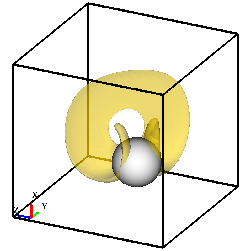
The Enright test is described in [62] and is a standard test for benchmarking level-set data structures and related numerical methods [51][63]. The test is straightforward to setup: A sphere with radius  is placed with its center at
 ![\( \bm {x}=[0.35,0.35,0.35] \)](lateximages/4E9C9B706FA6E74487CC7B2553B19427.svg) . The simulation domain is the unit box:
. The simulation domain is the unit box: ![\( [0,0,0] \)](lateximages/1E9339D21D1B7123F77DF8F216112A6B.svg) to
to ![\( [1,1,1] \)](lateximages/D1CFA157D05274C828571CF2D9CEBB68.svg) (cf. Figure 3.8). The velocity field
(cf. Figure 3.8). The velocity field  is a three-dimensional incompressible flow field modulated with a
period
is a three-dimensional incompressible flow field modulated with a
period  , i.e., a multiplication with
  , which results in
![(3.13) \{begin}{align} \label {eq:enrightfield} \bm {V}(\bm {x},t) = \begin {bmatrix} \cos (t\frac {\pi }{3}) [2 \sin ^2(2\pi x)\sin (2xy)\sin (2\pi z)] \\ \cos (t\frac {\pi }{3})
[-\sin (2\pi x)\sin ^2(\pi y) \sin (2\pi z)] \\ \cos (t\frac {\pi }{3}) [-\sin (2\pi x)\sin (2\pi y)\sin ^2(\pi z)] \end {bmatrix} \ . \{end}{align}](lateximages/lateximage-331.svg)
The sphere is mangled through this velocity field resulting in a very thin structure at  where the velocity field and thus the deformation as well is reversed (due to the temporal cosine
modulation). The analytical result is again the original structure (sphere) for
where the velocity field and thus the deformation as well is reversed (due to the temporal cosine
modulation). The analytical result is again the original structure (sphere) for  .
.
In Appendix A.1, Figure A.1-A.4 illustrate
the deformed states of the sphere from  to for various resolutions. For the lowest resolution (
 , Figure A.4) the thin regions are not
representable from
, Figure A.4) the thin regions are not
representable from  onwards (cf. Section 3.1),
leading to a drastic loss in volume at the final time . When the resolution in is increased (cf. Figure A.1-Figure A.3), the loss in volume is decreased.
onwards (cf. Section 3.1),
leading to a drastic loss in volume at the final time . When the resolution in is increased (cf. Figure A.1-Figure A.3), the loss in volume is decreased.
Table 3.1 shows the results using the OpenVDB data structure to store the level-set and performing the surface advection using a TVD-RK3 time integration scheme and WENO schemes for spatial discretization; three iterations (i.e., time steps) of a flow-based normalization are performed after the advection using the same WENO schemes and a TVD-RK1 time integration.
| Domain resolution | Memory [MB] | Advection [s] | Performance [MAV/s] | Active voxels [million] |
|
0.6/1.0 | 0.01/0.03 | 2.3/2.8 | 0.027/0.078 |
 |
1.6/4.3 | 0.04/0.13 | 2.7/3.0 | 0.11/0.39 |
 |
5.4/18 | 0.15/0.56 | 2.9/3.1 | 0.44/1.7 |
 |
20/76 | 0.57/2.4 | 2.9/3.1 | 1.7/7.2 |
 |
80/330 | 2.4/10 | 2.9/3.1 | 7.1/29 |
Table 3.1: Performance characteristics for the Enright test for resolutions from to (min/max) test on WS1 (cf. Section 3.4).
Column 1: Memory footprint of the VDB data structure (single-precision floating point representation). Column 2: Time for the advection step (TVD-RK3, WENO) including normalization (3 iterations, flow-based TVD-RK1, WENO) and tracking
of the narrow band. Column 3: Advection performance in MAV/s (million active voxels per second). Column 4: Number of active voxels.
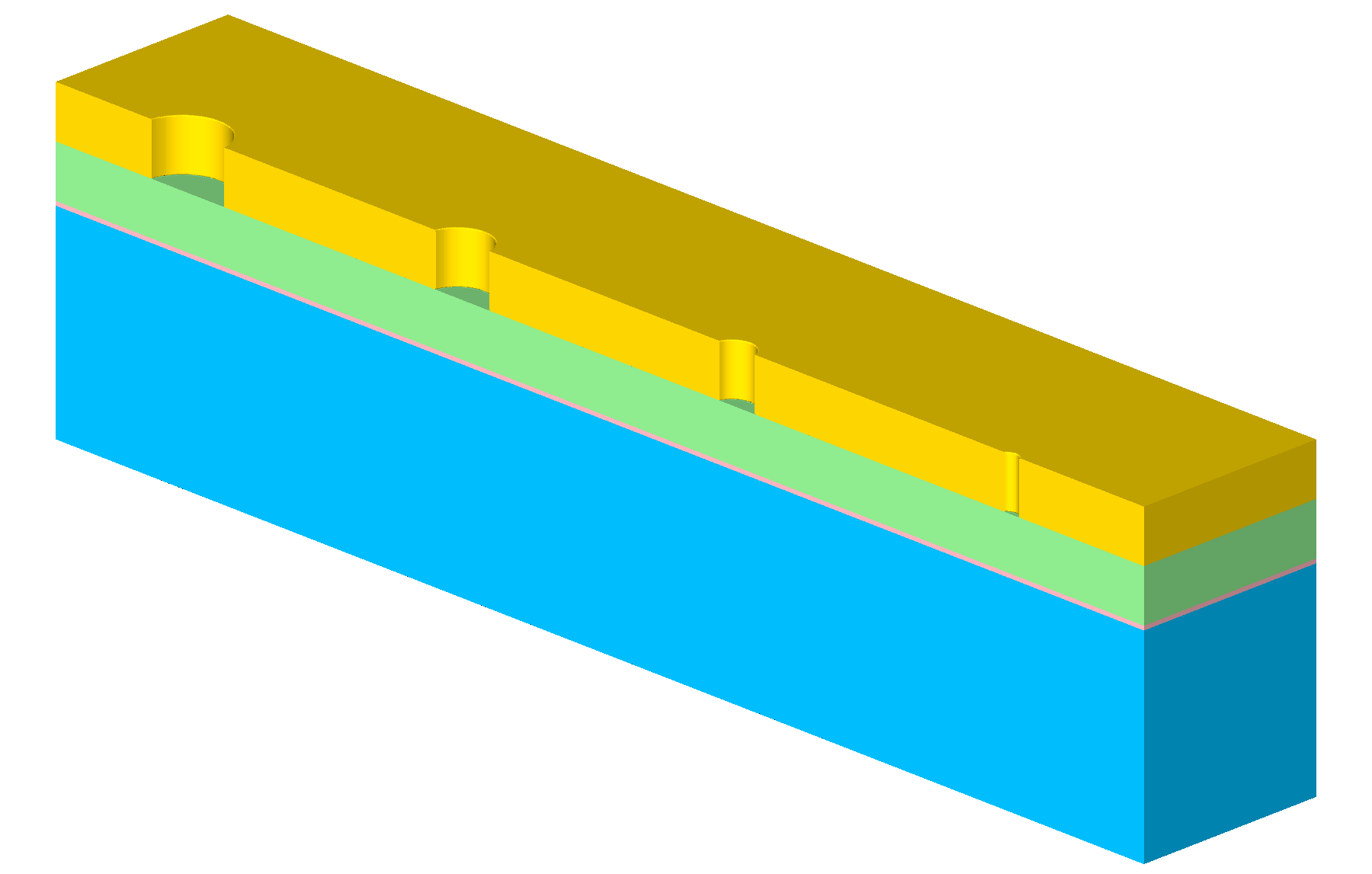
Material Dependent Isotropic Etching
The test configuration (isotropic test) consists of four stacked layers of different materials  . The surface velocity model is an isotropic etch rate:

The lateral domain dimensions are  (cf. Figure 3.9). The boundary conditions are reflective in both lateral directions. The thicknesses of the layers from top to bottom are
  (
( ), (
), ( ),
),  (
( ), and
  (
( ), respectively. The top layer () has four cylindrical holes of varying diameters
  ,
,  ,
,  , and
, and  . The centers are located on one of the longer lateral boundaries of the domain and are equidistantly spaced
with a distance of
. The centers are located on one of the longer lateral boundaries of the domain and are equidistantly spaced
with a distance of  .
.
Three different level-set resolutions were used:  ,
,  , and
, and  , corresponding to lateral dimensions of
  ,
,  , and
, and  grid cells for the simulation domain. The simulation is run until time
 using a TVD-RK3 time integration scheme with
  . The simulation results for
 ![\( T=[0,1] \)](lateximages/7E97FB732E0051D52E4244BC872AFD72.svg) are illustrated in Figures A.5-A.7. The thin material layer () has a low etch rate compared to the materials above and below; for the lowest
resolution (
are illustrated in Figures A.5-A.7. The thin material layer () has a low etch rate compared to the materials above and below; for the lowest
resolution ( ) the layer is just a bit thicker than one grid cell. Nevertheless, the
multi-material level-set representation described above allows to represent this thin layer with sub-grid thickness (cf. Section 3.1) during the level-set advection.
) the layer is just a bit thicker than one grid cell. Nevertheless, the
multi-material level-set representation described above allows to represent this thin layer with sub-grid thickness (cf. Section 3.1) during the level-set advection.
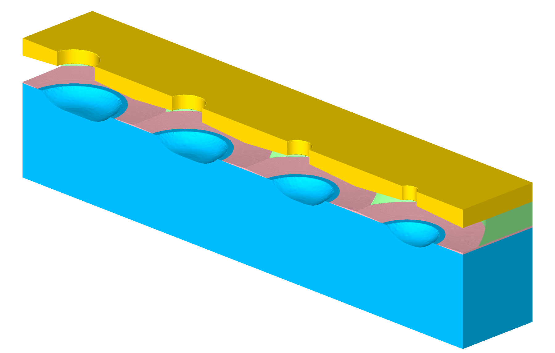
If the material regions are reconstructed from the multi-material level-sets (using Boolean operations), the thin layer vanishes in regions where no grid cell center is situated between the wrapping level-sets. This effect is visualized in
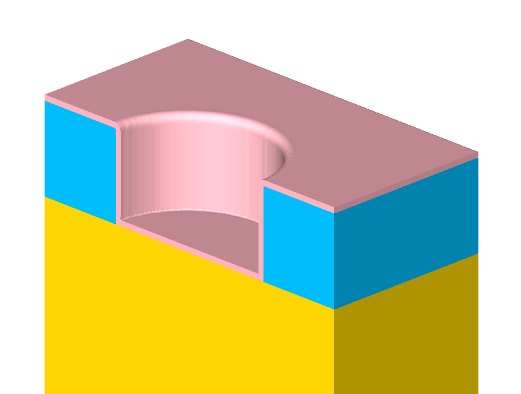
Figure 3.10 where this sub-grid resolution is shown for the thin layer of near the crater in at  .
.

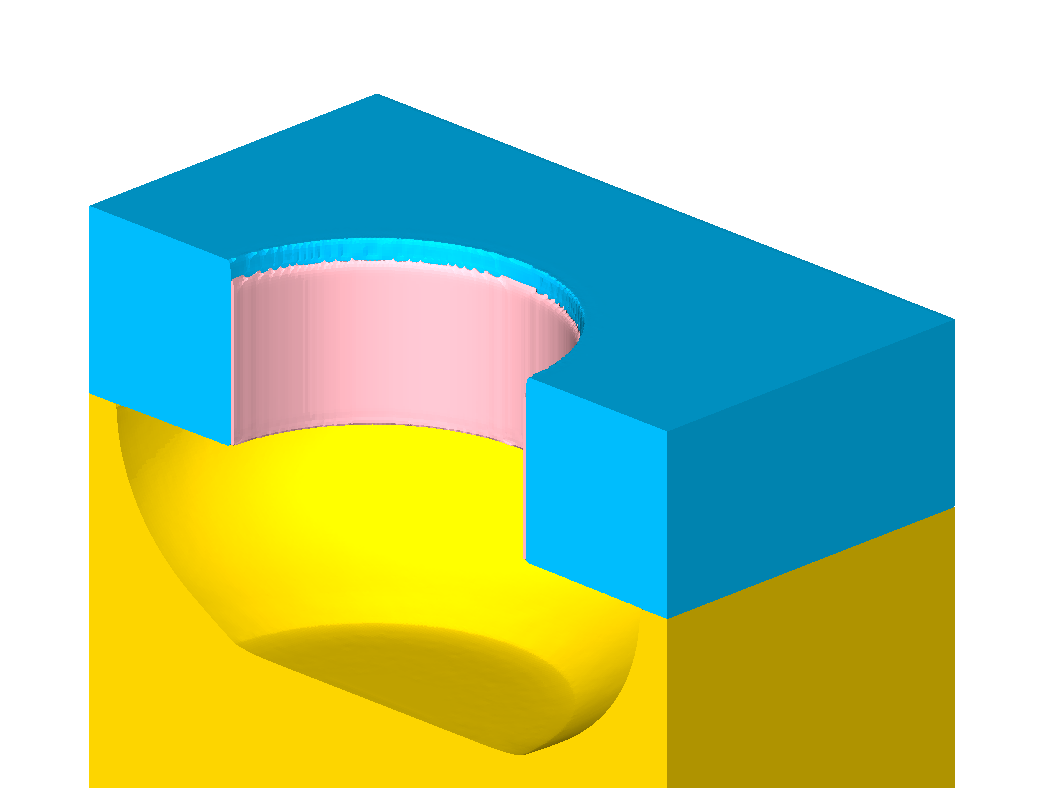
Figure 3.10: Material regions at  for the rightmost hole. (a) The explicit representation of the top layer level-set is shown (red triangle
mesh). (b) A spot near the crater in material is magnified to illustrate the sub-grid resolution of the thin material later (). If no grid cell is between the two wrapping level-sets, the thin layer vanished
during a Boolean operation between the wrapping level-sets. This is visible in the horizontal region near the crater. Nevertheless, the layer is still represented through the wrapping level-sets and considered during the surface advection.
for the rightmost hole. (a) The explicit representation of the top layer level-set is shown (red triangle
mesh). (b) A spot near the crater in material is magnified to illustrate the sub-grid resolution of the thin material later (). If no grid cell is between the two wrapping level-sets, the thin layer vanished
during a Boolean operation between the wrapping level-sets. This is visible in the horizontal region near the crater. Nevertheless, the layer is still represented through the wrapping level-sets and considered during the surface advection.
Figure 3.11 shows the cross section for the hole of diameter at different simulation times for all three resolutions. The low etch rate of slows etching in the downward direction, until the thin layer is first opened at
the center line of the hole.


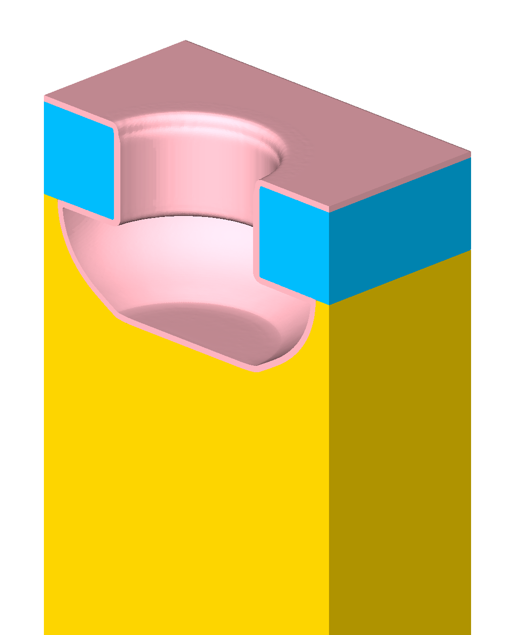
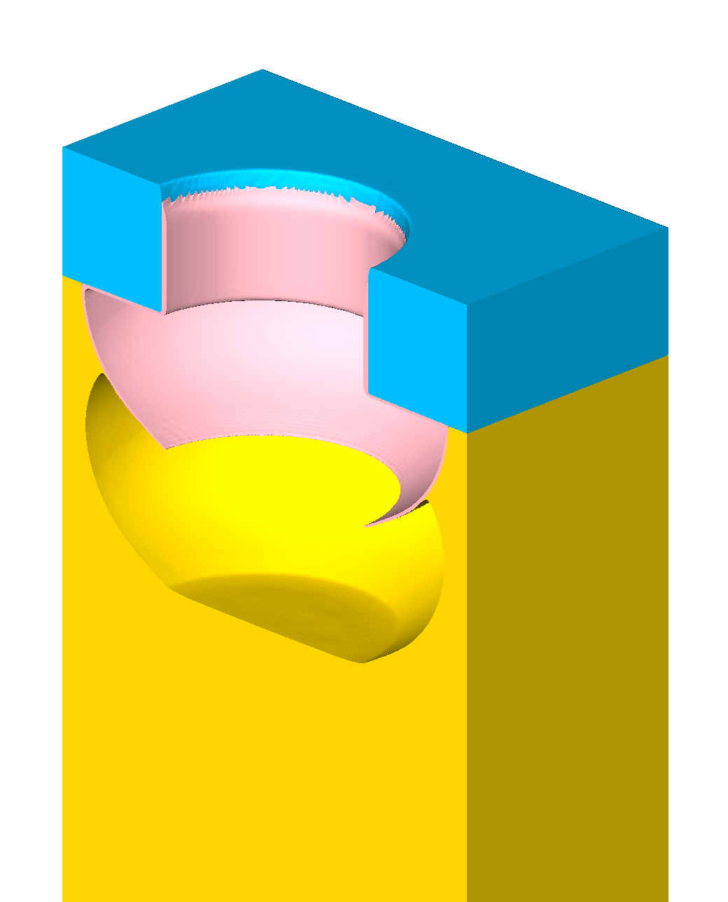
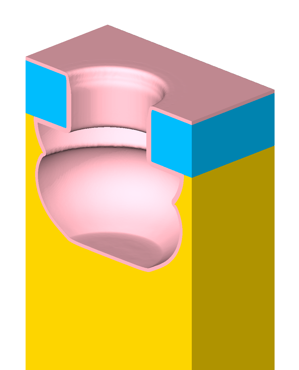
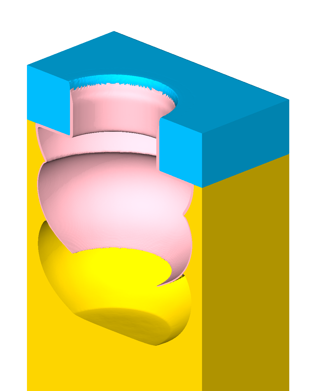
Simple Bosch Process
The Bosch process is a technique to fabricate high aspect ratio structures which are obtained by alternating a passivation step with an etching step. The passivation layer protects the sidewalls in the following directional etching step. In the etching step, accelerated ions remove the passivation layer primarily on horizontal surface regions, i.e., at the open top surface and the bottom of the structure. Once the passivation layer is removed at the bottom, the substrate is also etched isotropically by a neutral etchant species.
For this test case (Bosch test), etching and deposition are assumed to be isotropic and the accelerated ions are modeled to have perfect vertical trajectories. No re-emissions are considered allowing to simplify modeling the ion flux by a single vertical (upward) visibility check weighted with the projected surface area. This simple model is deliberately chosen as this test case is solely conducted to evaluate the capabilities of the framework.
The involved materials are a mask  patterned with the desired structure, a substrate
  into which the pattern is transferred, and a passivation material
  . This results in an isotropic surface velocity for the deposition of the
passivation layer
. This results in an isotropic surface velocity for the deposition of the
passivation layer

and a combined (isotropic and directed) surface velocity for the etching step

where  is the surface normal direction and
  is an upward unit vector. The second summand is only
considered, if the upward visibility check (a single upward ray is traced) evaluates to false, i.e., the source is visible. The duration of the passivation step is
is an upward unit vector. The second summand is only
considered, if the upward visibility check (a single upward ray is traced) evaluates to false, i.e., the source is visible. The duration of the passivation step is  and the duration of the etching step is
  . The simulation of 20 cycles is conducted using a domain with lateral dimensions
  and reflective boundary conditions. A mask () of thickness is patterned with a cylindrical hole of radius with its center midway on one of the longer domain boundaries.
Figure 3.12 illustrates the results of the first 5 processing steps.
The results for all 20 cycles are provided in Figures A.8-A.11 in Appendix A.3 for resolutions , , , and  . It becomes apparent that the sub-grid resolution of thin layers is essential
especially at low resolutions, as the thin passivation layer would not be representable otherwise.
. It becomes apparent that the sub-grid resolution of thin layers is essential
especially at low resolutions, as the thin passivation layer would not be representable otherwise.
Figure 3.13 compares the final results for four different resolutions. Larger differences in the absolute position of the side wall are noticeable for the lower resolutions.


3.4 Benchmarks
The individual computational tasks of the simulation platform were benchmarked on two hardware configurations:
Workstation 1 (WS1). Intel Core-i7-4790K system, 4 physical cores (8 logical cores),  MB of shared L3 cache,
  GB of main memory.
Workstation 2 (WS2)2. Dual CPU Intel Xeon E5-2650v2 system, each CPU has 8 physical cores (16 logical cores),  MB of L3 Cache, 64GB of main memory.
Utilizing all available cores (including hyper-threading), the isotropic test is benchmarked on WS1: The runtime of the main computational tasks (resolution ) is shown in Figure 3.14. The majority of runtime is utilized by the surface advection. The second largest runtime is used for the surface representation, which includes the extraction of an explicit
surface of the top layer level-set and the detection of the active layer for each triangle of the top layer. The runtime per time step doubles throughout the simulation. This increase is due to the increasing surface area; from  onwards, the surface area and consequently the runtime decreases.
Figure 3.15 shows the runtime of the main computational tasks throughout the simulation of the Bosch test: Also here, the dominating runtime during the deposition steps is the surface advection. During the etching steps the surface representation and the surface rates increase: The active material region must be determined leading to a larger runtime for the surface representation, and the upward visibility test effects the runtime for the surface rates.

Figure 3.14: Runtime of the main computational tasks for all time steps ( to ) of the isotropic test illustrated in Figure A.5.
The lateral resolution of the domain is . At the top, the corresponding cross sections of the domain are
shown for times
to ) of the isotropic test illustrated in Figure A.5.
The lateral resolution of the domain is . At the top, the corresponding cross sections of the domain are
shown for times  , and
, and  . The simulation was performed on WS1.

Figure 3.15: Runtime of the main computational tasks for all time steps ( to  ) of the Bosch test illustrated in Figure A.8.
The lateral resolution of the domain is
) of the Bosch test illustrated in Figure A.8.
The lateral resolution of the domain is  . At the top, the corresponding cross sections of the domain are shown
after cycle 1 (
. At the top, the corresponding cross sections of the domain are shown
after cycle 1 ( ), cycle 5 (
 ), cycle 10 (
 ), and cycle 20 (). The simulation was performed on WS1.
To evaluate the parallel scalability of the surface advection, the first time steps of the Enright test for resolution (7.1 MAV), the isotropic test for resolution (7.0 MAV), and the Bosch test for resolution (0.5 MAV) were benchmarked on a 16-core WS2. Figure 3.16 illustrates the results for up to 32 threads: The speedups are 12, 10, and 7.5 for 16 threads, respectively.

2 Represents a single node on the Vienna Scientific Cluster 3 (VSC-3); https://vsc.ac.at
3.5 Summary
The developed simulation platform provides important features to validate new approaches for the particle transport calculation: Multi-material advection, sub-grid resolution of thin layers, periodic and reflective boundary conditions, and an interface for efficient ray-surface intersections using external libraries. These features allow to qualify new approaches for the particle transport using realistic simulation setups. The surface advection shows appropriate speedup on shared-memory systems, although the scalability of the surface advection is not primarily important (as the focus is on the performance of the particle transport), it is advantageously as a realistic distribution of runtime between the individual computational tasks is obtained.
The platform is used to implement and validate the numerical approaches in the following Chapters 4, 5, and 6, respectively.