6 Sparse Evaluation of Surface Velocities
A constant spatial resolution throughout the domain is a straightforward choice for feature-scale process simulation. An advantage is that numerical schemes for advection and extraction algorithms can be applied without the need to consider multiple resolutions. Another advantage is that geometric features are represented in the full domain with maximum accuracy. For high spatial resolutions, this results in a highly resolved surface representation which is used during the particle transport calculation. In a straightforward approach, the surface rates are evaluated using the full resolution of the surface. This represents a valid and robust approach as the surface advection is conducted with maximum spatial accuracy. The particle transport is typically dominating the runtime of the simulation in such cases.
The material surfaces potentially experience very different advection rates, depending on the simulated process and the geometric configuration. For instance, a large portion of the fully exposed horizontal surface of a photoresist is advected with a constant vertical velocity. Other regions of the surface potentially exhibit locally very different advection rates, e.g., in regions near the transition from a vertical to horizontal surface orientation.
Considering the resulting different requirements for spatial resolutions, one approach is to reduce the overall computational complexity by locally reducing the spatial resolution (of the level-set) in regions where it is admissible without sacrificing the advection accuracy. Within the scope of the example discussed above, a lower spatial resolution is used for the top surface of the photoresist. Approaches based on a local spatial reduction of the resolution cannot solely rely on the geometrical properties of the surface: Local variations of the advection rate might also occur on planar material surfaces due to shadowing from remote regions of the surface. That is, depending on the local surface advection rates, the level-set resolution has to be re-adopted accordingly, e.g., to capture features of the geometry which develop in previously planar regions.
The approach presented in the following is based on a constant spatial resolution of the level-set function [3]. The computational complexity is reduced by selecting a sparse set of points on the surface. The surface rates are evaluated only
on this sparse set leading to a reduction of the computational demand of the direct flux calculation. This sparse set of points is generated according to application-specific requirements with an iterative partitioning scheme: The local geometrical
properties and local deviation of the direct flux are used to locally define the resolution of the sparse points. The flux rates at the sparse points are also applied in the neighborhood which is assigned to each sparse point. This constant
extrapolation is then “diffused” to obtain an approximation of a linear interpolation between these sparse points. Figure 6.1 demonstrates the approach for a
structure etched by the direct flux from a tilted focused particle source with direction ![\( [0.5,0.5,-1] \)](lateximages/788653F96D3194D8776865713BDC6049.svg) . The red triangles on the surface of Figure 6.1a and 6.1c depict the sparse set of points for which the surface rates are
evaluated. Figure 6.1b and 6.1d illustrate the corresponding direct
flux.
. The red triangles on the surface of Figure 6.1a and 6.1c depict the sparse set of points for which the surface rates are
evaluated. Figure 6.1b and 6.1d illustrate the corresponding direct
flux.
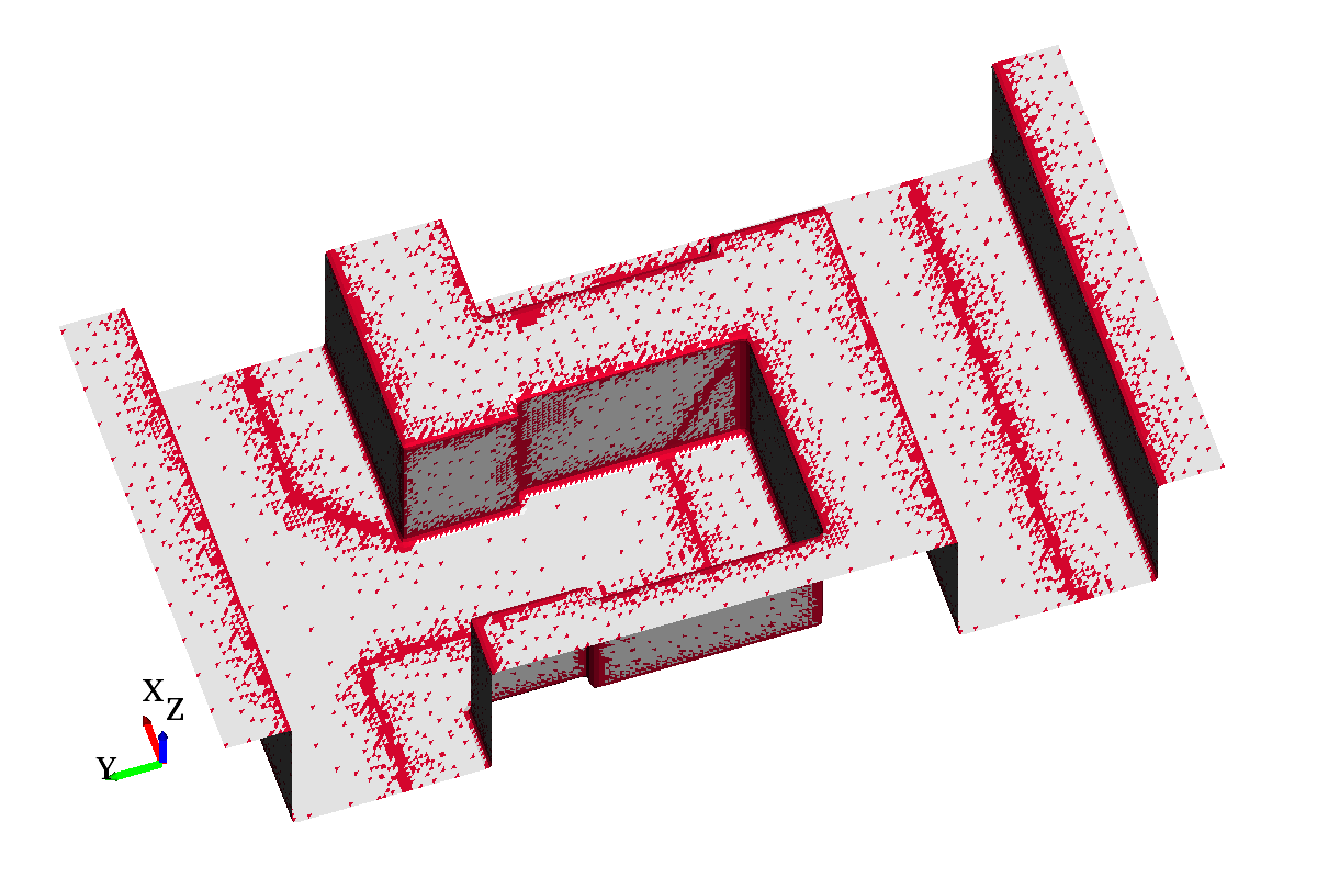
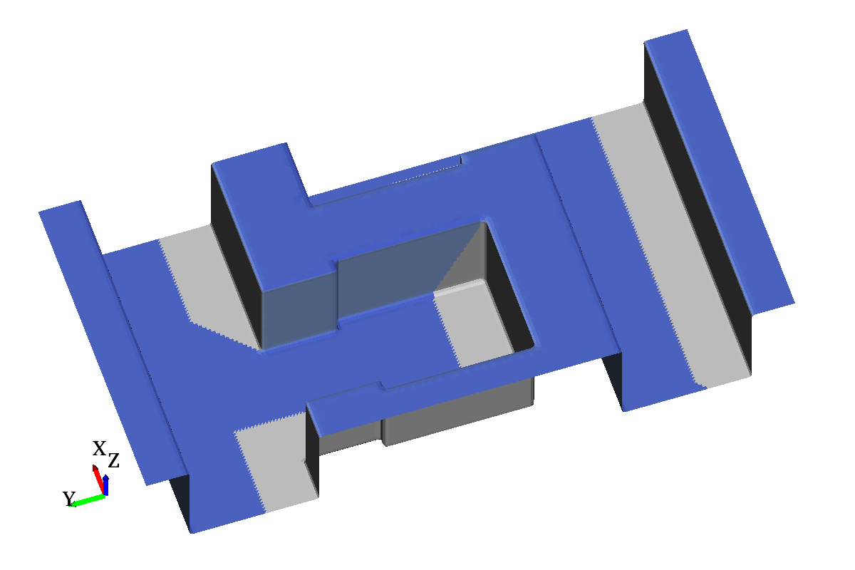
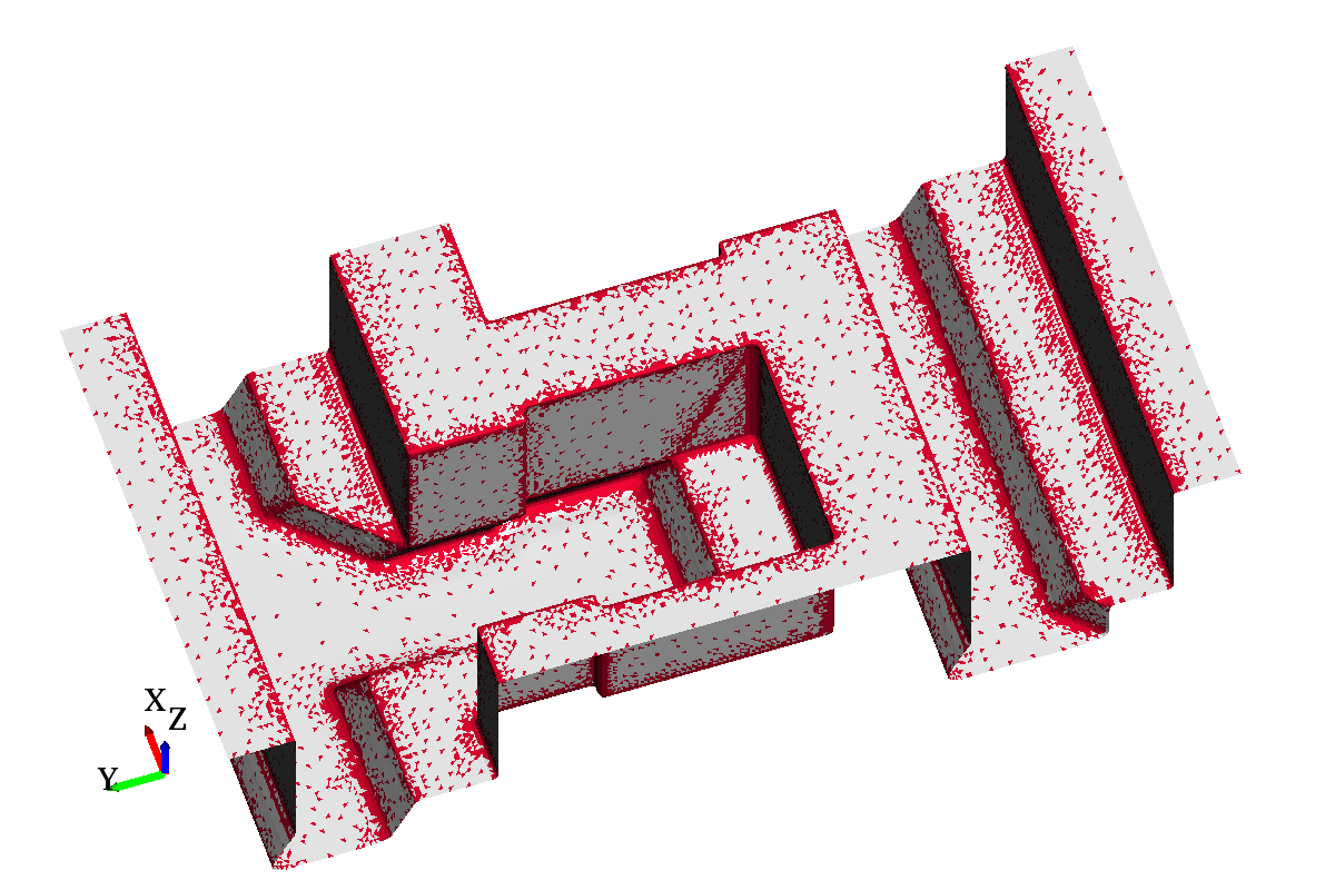
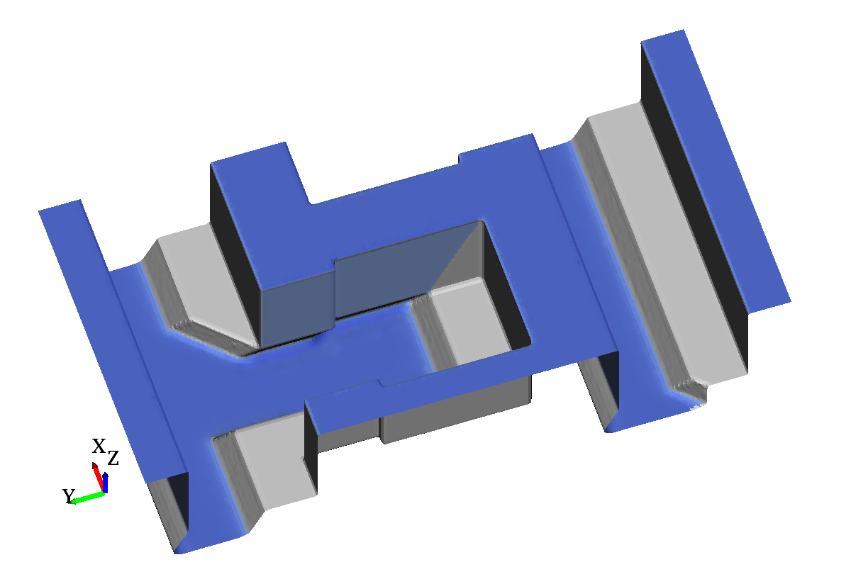
Figure 6.1: Top layer of a two-material etching simulation for a focused source with direction to demonstrate the result of the iterative partitioning scheme. The re-
sulting sparse set of points and corresponding direct flux for the initial geometry (a) (b)
and geometry and at a later etched stage (c) (d) is visualized. The blue color
in (b) and (d) encodes the received direct flux, whereas gray corresponds to shad-
owed regions, i.e., zero flux.
In the following, first the iterative partitioning scheme and the subsequent interpolation are introduced in detail. Then, the method and its performance is evaluated using different resolutions of a simple etching test case.
6.1 Iterative Partitioning Scheme
The scheme presented in the following provides a robust method to reduce the number of necessary evaluation points for which the surface rates are calculated. From a dense set of evaluation points given by the resolution of an explicit surface mesh, a subset of points is selected using an iterative partitioning scheme. The scheme is controlled by a freely definable refinement condition, allowing to adopt the method for different application-specific requirements (cf. Section 6.3).
The dense set of evaluation points is defined as the set of all triangle centroids. Algorithm 2 is used to iteratively select a sparse subset of
evaluation points depending on (a) the maximally globally allowed edge distance ( ) between two points in the subset, (b) an array of maximally allowed
edge distances for each point in the dense set where each entry is between 0 and , and (c) a refinement condition. The refinement condition defines in each
iteration and for each point in the sparse set, if additional points in the surrounding should be added to the sparse set. Algorithm 2 assigns one of the sparse
points to each of the points in the dense set: This way, a neighborhood is formed from all points with the same sparse “parent”. This neighborhood is referred to as patch in the following. The patches are the “spacers” between the points in
the sparse set and are used to efficiently identify neighbors in the sparse set and to generate the initial guess for the Jacobi solver discussed in Section 6.2. As will be
discussed later in more detail, the refinement condition used in Section 6.3 is based on a fixed threshold for the angular deviation of the surface normal and the
deviation of the direct flux (from a source) between a sparse point and its sparse neighbors. Details for the functions in Algorithm 2 can be found in
Appendix C.2.
) between two points in the subset, (b) an array of maximally allowed
edge distances for each point in the dense set where each entry is between 0 and , and (c) a refinement condition. The refinement condition defines in each
iteration and for each point in the sparse set, if additional points in the surrounding should be added to the sparse set. Algorithm 2 assigns one of the sparse
points to each of the points in the dense set: This way, a neighborhood is formed from all points with the same sparse “parent”. This neighborhood is referred to as patch in the following. The patches are the “spacers” between the points in
the sparse set and are used to efficiently identify neighbors in the sparse set and to generate the initial guess for the Jacobi solver discussed in Section 6.2. As will be
discussed later in more detail, the refinement condition used in Section 6.3 is based on a fixed threshold for the angular deviation of the surface normal and the
deviation of the direct flux (from a source) between a sparse point and its sparse neighbors. Details for the functions in Algorithm 2 can be found in
Appendix C.2.
Input:  , distTarget[
 ], RefinementCondition()
Output: active[], sparseNeighbors[], patches[]
Algorithm
withdrawn[ ] = true; reflagged[] = false; active[] = false;
distance[] = ; parent[] = -1;
patches[] = empty map(activeIndex,patchIndices);
sparseNeighbors[] = empty map(activeIndex,activeNeighbors);
indices[] = iota(0,);
FlagTriangles(indices,  )
)
RebuildPatches();
EvaluateSurfaceModel(for all active indices)
for n=1… ) do
) do
reflagged[] = false;
withdrawn[] = false;
numNewPatches = 0;
foreach  in patches do
 ;
;
if RefinementCondition( ) == true AND reflagged[] == false then
numNewPatches += RefinePatch(,  );
);
if numNewPatches == 0 then
break;
RebuildPatches();
EvaluateSurfaceModel(for all newly active indices)
Algorithm 2: Adaptive decimation of evaluation locations on a triangular surface mesh.
Figure 6.2 illustrates the individual stages of the algorithm using a small, regular triangle mesh.


Figure 6.2: Schematic depiction of the stages of the iterative partitioning scheme for an exemplary mesh. Yellow lines denote patch boundaries. (a) Initial creation of a
patch where the numbers refer to edge distances to the origin; for visualization purposes only, the triangles which will be removed from the patch in the next step use a smaller font size. (b)
Creation of a second patch (blue) starting at one of the unprocessed triangles. (c) Sparse neighbor connection between the two origins of the patches. (d)
Withdrawal of sub region in red patch. (e) Refinement of the withdrawn region in the red patch with  . (f)
Updated sparse neighbor connections after the red patch is refined.
. (f)
Updated sparse neighbor connections after the red patch is refined.
After the refinement is completed for all patches where the refinement condition evaluates to true, the refinement condition is re-evaluated for all sparse points. Subsequently, the refinement is repeated with  , continuously leading to a bisection of the maximal edge
distance between sparse points on the patch. The algorithm is terminated either because the refinement condition evaluates to false for all sparse points or
, continuously leading to a bisection of the maximal edge
distance between sparse points on the patch. The algorithm is terminated either because the refinement condition evaluates to false for all sparse points or  , corresponding to a patch consisting of only one triangle. If the
refinement condition depends on the surface velocity at the sparse points, the surface model must be evaluated for the newly added sparse points in each iteration. After completion, Algorithm 2 provides a sparse set of points with corresponding sparse neighbors and patch information.
, corresponding to a patch consisting of only one triangle. If the
refinement condition depends on the surface velocity at the sparse points, the surface model must be evaluated for the newly added sparse points in each iteration. After completion, Algorithm 2 provides a sparse set of points with corresponding sparse neighbors and patch information.
How well the edge distances between the sparse points map to arc length distances on the triangular mesh depends on the uniformity of the mesh with respect to triangle shape and size. Only with a mesh consisting of triangles with comparable size and quality the algorithm will produce “convex” patches (convex with respect to the projected polygon constructed of the outermost centroids).
Figure C.3 in Appendix C.1 demonstrates the resulting set of sparse points for each iteration
when using  for the two-material geometry introduced in Figure 6.1. The refinement condition (6.2) is employed and the
sparse set of points is initialized with the points near the material interfaces.
for the two-material geometry introduced in Figure 6.1. The refinement condition (6.2) is employed and the
sparse set of points is initialized with the points near the material interfaces.
6.2 Interpolation Between Sparse Points
Inherent to its construction method, the sparse set of points and the connections between sparse neighbors do not necessarily allow to construct a sparse mesh covering the complete original surface, which could be used for interpolation. To provide a robust, non-supervised, and computationally efficient interpolation between the sparse points, a constant extrapolation inside the patches using the corresponding values at the origins is performed, i.e., the values of the sparse points are assigned to the full corresponding patch. The properties of Laplace’s equation (6.1) and the error diffusion properties of the Jacobi method [5] are used to smooth the “jumps” in the constant extrapolation and to approximate a linear interpolation between the sparse points:
(a) In one dimension, the solution of Laplace’s equation (6.1) is equivalent to a linear interpolation between a sparse set of points when using the sparse set as Dirichlet boundary conditions and modeling the boundaries of the domain as Neumann boundary conditions.
(b) In one iteration of Jacobi’s method, local information propagates only across one edge; using this property the radius of influence is restricted to not exceed the maximal patch radius of  by only performing or less iterations.
A linear interpolation between the sparse points on the surface is approximated by using the same boundary conditions (as for the one-dimensional case mentioned above) and starting with the constant extrapolation as an initial guess. (6.1) is not solved until convergence but only a fixed number of iterations of Jacobi’s method is performed.

A finite volume approximation is used to discretize (6.1) on the triangulated mesh by

where  is the scalar function (in this case the local surface rate),
  is the length of the edge shared by triangle and
  ,
,  is the centroid of triangle , and
  is the centroid of the triangle connected to triangle across edge . This discretization and the boundary conditions described above results in a
system of linear equations. The number of unknowns is the number of all centroids minus the size of the sparse set.
is the centroid of the triangle connected to triangle across edge . This discretization and the boundary conditions described above results in a
system of linear equations. The number of unknowns is the number of all centroids minus the size of the sparse set.
6.3 Evaluation and Performance
The simulation platform described in Section 3 is used to implement, validate, and benchmark the approach. A generic etching simulation test case with a single material region is
used for the evaluation. The model for the surface velocity is a linear relation to the direct incident flux from a source with a power cosine distribution  , which is a common choice in Process
TCAD for the distribution of accelerated ions. The bottom-up integration method based on a subdivided icosahedron (cf. Section 4.1) is used to calculate
the direct flux rates on the surface. Here, a 5 times subdivided icosahedron is used to limit effects of the integration accuracy. The direct flux rates are normalized to the flux rate on a fully exposed horizontal plane.
, which is a common choice in Process
TCAD for the distribution of accelerated ions. The bottom-up integration method based on a subdivided icosahedron (cf. Section 4.1) is used to calculate
the direct flux rates on the surface. Here, a 5 times subdivided icosahedron is used to limit effects of the integration accuracy. The direct flux rates are normalized to the flux rate on a fully exposed horizontal plane.
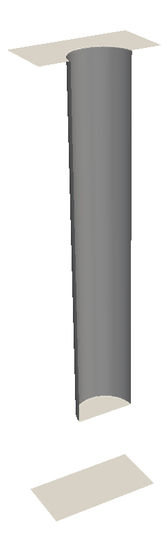
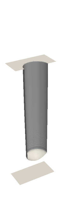
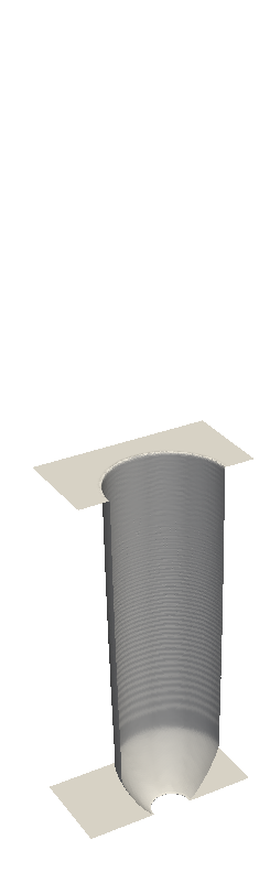
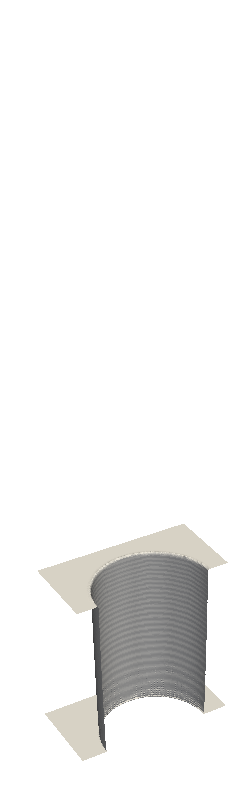
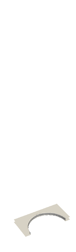
The initial geometry (Figure 6.3a) is a cylindrical hole with diameter 1 and depth 6 in a bulk region of thickness 8. Figure 6.3b-6.3e show the intermediate surface positions using the dense centroid-set for surface model evaluation (dense flux evaluation) from time T=0 up to T=8, where the bulk region is completely etched.

To model the refinement condition, for each sparse point

are defined, where  is the set of neighboring sparse point indices, and
  and
and  are the global maximum and minimum flux value, respectively. A
combination of fixed thresholds is used in all of the following results to model the refinement condition in Algorithm 2:
are the global maximum and minimum flux value, respectively. A
combination of fixed thresholds is used in all of the following results to model the refinement condition in Algorithm 2:

Furthermore,  is used in all simulations, which gives a total of 6 iterations (1 initial
iteration, and
is used in all simulations, which gives a total of 6 iterations (1 initial
iteration, and  refinements), whereas the number of Jacobi iterations is fixed to
 .
.
Figure 6.4 illustrates the resulting sparse centroid-set at time T=4.5 for different level-set resolutions. Analogously, Figure C.1 and C.2 in Appendix C illustrate the results for
 and
and  .
.
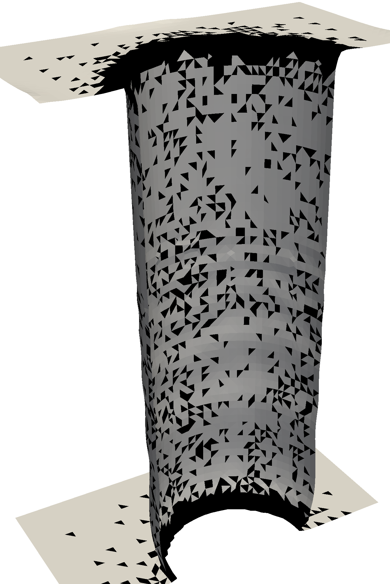

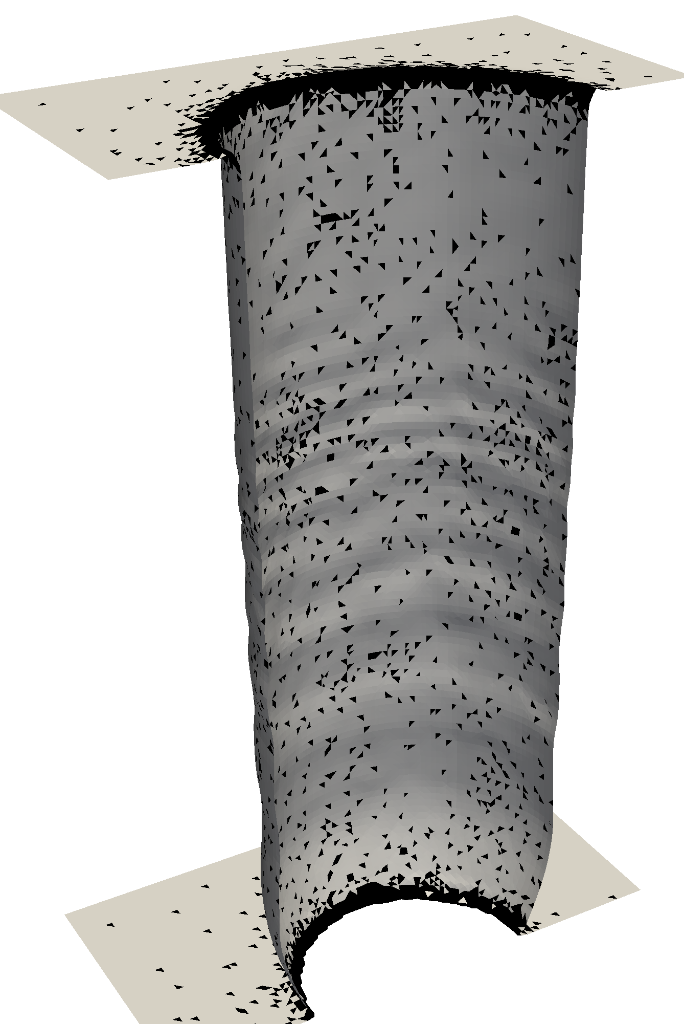

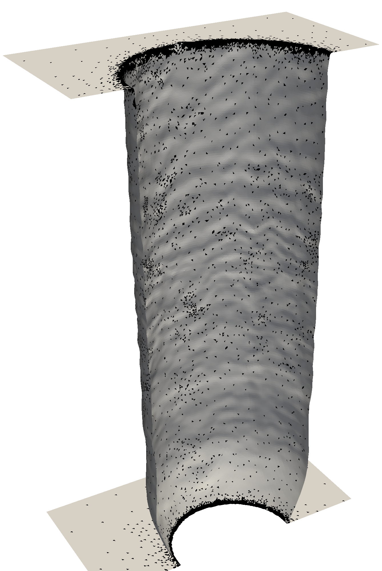

Figure 6.4: Sparse set of triangles (black; correspond to triangles which are labeled “0” in Figure 6.2) for level-set resolutions 16 (a), 32 (b), and 64 (c) at time T=4.5. The ratios between the total number of triangles and the sparse set of triangles are provided in the subcaptions. These ratios correspond to the dense/sparse ratios in Figure 6.7, 6.8, and 6.9.
In Figure 6.5, the results between the dense and sparse flux evaluation at times T=3 and T=6 are compared. For a level-set resolution of 64, this corresponds to time step 800 and 1600, respectively.

(a) Resolution 16

(b) Resolution 32

(c) Resolution 64
Figure 6.5: Comparison of surface positions at times T=[3,6] for all tested resolutions. The surface mesh for the dense and sparse flux evaluation is displayed on the left and right half-space, respectively. Two regions are magnified for resolution 64 where the blue and red line correspond to slices of the sparse and dense evaluation, respectively.
In Figure 6.6, the corresponding maximum deviations throughout the simulations are shown. The maximum deviations peak slightly below 3 level-set cell widths
( ). For resolution 32, the error stays below . In the upper region of the hole and the top surface, the deviations are small and the sharp edge is
conserved.
). For resolution 32, the error stays below . In the upper region of the hole and the top surface, the deviations are small and the sharp edge is
conserved.


The performance of the method is evaluated by tracing the runtime per time step from T=0 to T=8 for three different level-set resolutions summarized in Table 6.1 for the dense and the sparse flux calculation.
Table 6.1: Level-set resolutions, resulting initial domain resolutions, initial mesh properties, and resulting number of time steps until T=8.
| Cells per unit length | Cells vertical | Cells horizontal | Triangles | Time steps |
| 16 | 128 | 32x32 | 17k | 540 |
| 32 | 256 | 64x64 | 67k | 1080 |
| 64 | 512 | 128x128 | 262k | 2160 |
For each time step, the runtime for the flux evaluation and for the remaining parts (velocity extension, advection, normalization, and mesh extraction; referred to as other tasks in the following) is tracked (cf. Figure 6.7-6.9 green and red areas, respectively). The flux integration method for a single point is identical for both cases. The implementation of Algorithm 2 is serial, in contrast to the flux evaluation, which is OpenMP-parallelized in both cases to provide a realistic estimation of the speedups. The serial overhead generated by Algorithm 2 is captured in the runtime of the flux evaluation. All performance measurements were performed on WS1.
Figure 6.7 summarizes the performance differences for resolution 16. The left plot shows the runtime per time step for the dense flux evaluation. The runtime at the
beginning of the simulation is  seconds per time step. As soon as the hole has reached the bottom of the bulk material, the number
of triangles starts to decrease and consequently the runtime per time step drops linearly from T=3.6 to T=8. The ratio between flux evaluation (green) and other tasks (red) is
seconds per time step. As soon as the hole has reached the bottom of the bulk material, the number
of triangles starts to decrease and consequently the runtime per time step drops linearly from T=3.6 to T=8. The ratio between flux evaluation (green) and other tasks (red) is  for the whole simulation, emphasizing the dominance of the computational cost for the flux
evaluation, even for small domain resolutions. The right plot in Figure 6.7 is analogous to the left plot, but for the sparse flux evaluation. A second y-axis on the right is
used to plot two additional properties, namely: The ratio of dense to sparse points (dashed line) and the speedup of the flux evaluation (solid line) over the dense flux evaluation. Throughout the simulation, the dense/sparse ratio is between 2.5
and 6 while the speedup is
for the whole simulation, emphasizing the dominance of the computational cost for the flux
evaluation, even for small domain resolutions. The right plot in Figure 6.7 is analogous to the left plot, but for the sparse flux evaluation. A second y-axis on the right is
used to plot two additional properties, namely: The ratio of dense to sparse points (dashed line) and the speedup of the flux evaluation (solid line) over the dense flux evaluation. Throughout the simulation, the dense/sparse ratio is between 2.5
and 6 while the speedup is  .
.

Figure 6.8 and 6.9 compare the performance for resolution 32 and 64, respectively. With increasing resolution, the dominance of the flux evaluation in terms of runtime is also increased, leading to a negligible share of runtime for the other tasks in the case of dense flux evaluation. For sparse flux evaluation a dense/sparse ratio of 3 to 14 and 4 to 35 is achieved for resolution 32 and 64, respectively. However, different to resolution 16, the obtained speedups (5 and 8, respectively) are only constant up to T=3.6, where the hole reaches the bottom of the bulk material. From T=3.6 to T=8 the speedups decrease to approximately 2 (following the dense/sparse ratio) keeping the total runtime per time step approximately constant up to T=6.5.


The difference between achieved and potential speedup (i.e., dense/sparse ratio) is higher for large meshes and ranges from  for resolution 16, to
  for resolution 64 before the hole reaches the bottom. When approaching T=8, all three tested
resolutions converge to a speedup of .
for resolution 64 before the hole reaches the bottom. When approaching T=8, all three tested
resolutions converge to a speedup of .
6.4 Summary
A method was presented to reduce the number of necessary evaluation locations for the surface rates to reduce the computational effort with limited impact on the accuracy. A sparse point-set and corresponding neighborhoods are constructed using an iterative partitioning scheme. The surface rates are only evaluated for this sparse point-set. The variable limits for the allowed distance between sparse locations enable to balance between computational complexity and accuracy in a robust way. A linear interpolation between the sparse points is approximated by diffusing the result of a constant extrapolation in the neighborhoods.
When using a cylindrical hole with a directed vertical source as a generic etching simulation test case, deviations in the surface position are below 3 level-set cells for all tested configurations. The achieved speedups range from 2 for the lowest resolution up to 8 for the highest resolved surface. The speedups are tracked during all time steps of the simulations starting from thick initial geometries to very thin geometries at the end of the simulated physical process.