8 Combining Acceleration Techniques for Direct Flux
The approaches to accelerate the flux calculation presented in Chapters 4, 5, and 6 are applied to the etching simulation of a dielectric layer
introduced in Section 1.2 to showcase the advantage of their combined use. The surface velocity  is defined as a linear relation to the direct flux
  from a power cosine source (cf. Figure 4.3) with exponent
  .
.

The etching is simulated until  , where the etchstop embedded in the dielectric and the diffusion barrier is reached at
  and
and  , respectively; Figure 8.1a-8.1c show the corresponding
cross sections of the simulation domain.
, respectively; Figure 8.1a-8.1c show the corresponding
cross sections of the simulation domain.
All benchmarks in this chapter are performed on WS2. As a frame of reference, for resolution  , the runtimes of the main computational tasks with a 4 times subdivided
icosahedron for spherical sampling (cf. Section 4.1) and implicit ray tracing (using OpenVDB) are shown in Figure 8.1d. Analogously, Figure 8.1e shows the runtimes for the same setup, when applying the presented acceleration schemes, namely (a) explicit ray tracing on a
temporary explicit mesh (using Embree, cf. Section 5.3), (b) an adaptive sampling of the visibility directions with one level of
refinement (i.e., minlevel
, the runtimes of the main computational tasks with a 4 times subdivided
icosahedron for spherical sampling (cf. Section 4.1) and implicit ray tracing (using OpenVDB) are shown in Figure 8.1d. Analogously, Figure 8.1e shows the runtimes for the same setup, when applying the presented acceleration schemes, namely (a) explicit ray tracing on a
temporary explicit mesh (using Embree, cf. Section 5.3), (b) an adaptive sampling of the visibility directions with one level of
refinement (i.e., minlevel and maxlevel
 , cf. Section 4.3), and (c) a
sparse evaluation of the surface rates using a maximum edge distance of 16 (i.e.,
, cf. Section 4.3), and (c) a
sparse evaluation of the surface rates using a maximum edge distance of 16 (i.e.,  , cf. Section 6.1) and Equation (6.2) as refinement condition.
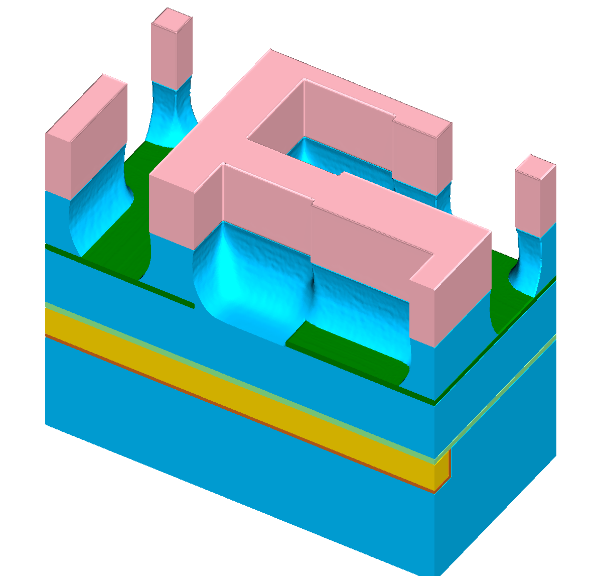
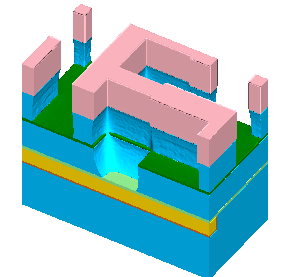
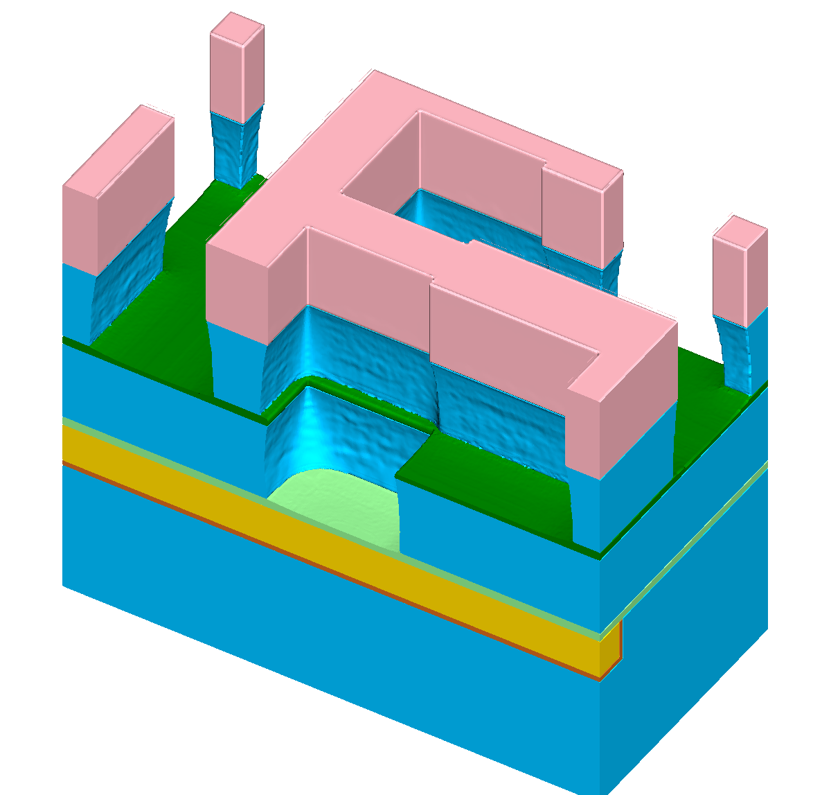


Figure 8.1: Results of a feature-scale etching simulation of the dielectric layer in a “self-aligned dual-damascene process” (cf. Figure 1.1h). The lateral dimensions of the domain
are  grid cells. (a)-
(c) Cross sections of the domain for
grid cells. (a)-
(c) Cross sections of the domain for ![\( T=[0.5,1.0,1.5] \)](lateximages/16C917D73083166CEFE056353577D5A0.svg) . (d)
Runtimes demanded with implicit tracing. (e) Runtimes using all presented acceleration approaches combined.
. (d)
Runtimes demanded with implicit tracing. (e) Runtimes using all presented acceleration approaches combined.
The overall runtime for a time step is about 70 seconds at the beginning of the simulation and about 110 seconds for . When applying all presented approaches combined the overall runtime is reduced to about 5 and 8 seconds,
respectively. This corresponds to an overall speedup of about 14.
The speedup for the calculation of the surface rates is shown in Figure 8.2 for various additional combinations of the presented acceleration approaches. The speedups are normalized to runtimes based only on an explicit ray tracing approach. The configurations corresponding to the result shown in Figure 8.1d and 8.1e are additionally marked with a circle.


Figure 8.2: Average speedup for the surface rate calculation for various combinations of the presented acceleration approaches normalized to the runtime with solely the explicit tracing approach (expl.). (a)
and (b) show the results for resolution 1/64 and 1/128, where the configurations are otherwise identical besides the  setting for the sparse evaluation of 16 and 32, respectively. The re-
sults corresponding to Figure 8.1d and 8.1e
are additionally marked with a circle in (a). The speedup with a top-down Monte Carlo approach for the direct flux is plotted in dashed lines where
each line represents a constant number of launched rays, i.e., 1k/tri corresponds to 1000 triangles launched per triangle on an equivalent horizontal surface.
setting for the sparse evaluation of 16 and 32, respectively. The re-
sults corresponding to Figure 8.1d and 8.1e
are additionally marked with a circle in (a). The speedup with a top-down Monte Carlo approach for the direct flux is plotted in dashed lines where
each line represents a constant number of launched rays, i.e., 1k/tri corresponds to 1000 triangles launched per triangle on an equivalent horizontal surface.
Figure 8.2 confirms the speedups estimated in the individual chapters presenting the acceleration approaches: The explicit ray tracing (which is used as a baseline, thick blue line) provides a speedup of about 9 compared to the implicit tracing (green line). The adaptive visibility sampling provides a speedup of 2 for a 6 times subdivided icosahedron; for lower subdivision levels, the speedup decreases to only a marginal speedup for 3 subdivisions. The sparse evaluation of the surface rates provides a speedup of 1.5 and 2 for 4 subdivisions up to 4.5 and 8 for 6 subdivisions. The combined speedup can be approximated by the product of the individual speedups. The speedup for the combined approaches is above 14 for 4 or more subdivisions.
Figure 8.2 additionally plots the speedups when using explicit tracing combined with a top-down Monte Carlo approach for the direct flux
calculation. The speedups are plotted for four different numbers of launched rays per triangle on a equivalent horizontal surface, i.e., for resolution 1/64 the launched number of rays is  Mrays, where 2 triangles are
assumed per grid cell and 1000 rays are launched per triangle (1k/tri).
Mrays, where 2 triangles are
assumed per grid cell and 1000 rays are launched per triangle (1k/tri).
Figure 8.2 also allows to relate the runtime between top-down and bottom-up approaches for the direct flux calculation, e.g., for resolution 1/64 the runtime for a top-down scheme using 1k/tri is about a factor of 0.7 slower than a sampling using a 4 times subdivided icosahedron. This relation can merely be used as a rough estimate as it strongly depends on the geometry, if the number of launched rays is related to the number of equivalent triangles of a horizontal surface.