[ Previous ] [ Home ] [ Next ]

Numerical Analysis and Innovative Simulation
Techniques for Designing Advanced MRAM

\(\newcommand{\footnotename}{footnote}\) \(\def \LWRfootnote {1}\) \(\newcommand {\footnote }[2][\LWRfootnote ]{{}^{\mathrm {#1}}}\) \(\newcommand {\footnotemark }[1][\LWRfootnote ]{{}^{\mathrm {#1}}}\) \(\let \LWRorighspace \hspace \) \(\renewcommand {\hspace }{\ifstar \LWRorighspace \LWRorighspace }\) \(\newcommand {\TextOrMath }[2]{#2}\) \(\newcommand {\mathnormal }[1]{{#1}}\) \(\newcommand \ensuremath [1]{#1}\) \(\newcommand {\LWRframebox }[2][]{\fbox {#2}} \newcommand {\framebox }[1][]{\LWRframebox } \) \(\newcommand {\setlength }[2]{}\) \(\newcommand {\addtolength }[2]{}\) \(\newcommand {\setcounter }[2]{}\) \(\newcommand {\addtocounter }[2]{}\) \(\newcommand {\arabic }[1]{}\) \(\newcommand {\number }[1]{}\) \(\newcommand {\noalign }[1]{\text {#1}\notag \\}\) \(\newcommand {\cline }[1]{}\) \(\newcommand {\directlua }[1]{\text {(directlua)}}\) \(\newcommand {\luatexdirectlua }[1]{\text {(directlua)}}\) \(\newcommand {\protect }{}\) \(\def \LWRabsorbnumber #1 {}\) \(\def \LWRabsorbquotenumber "#1 {}\) \(\newcommand {\LWRabsorboption }[1][]{}\) \(\newcommand {\LWRabsorbtwooptions }[1][]{\LWRabsorboption }\) \(\def \mathchar {\ifnextchar "\LWRabsorbquotenumber \LWRabsorbnumber }\) \(\def \mathcode #1={\mathchar }\) \(\let \delcode \mathcode \) \(\let \delimiter \mathchar \) \(\def \oe {\unicode {x0153}}\) \(\def \OE {\unicode {x0152}}\) \(\def \ae {\unicode {x00E6}}\) \(\def \AE {\unicode {x00C6}}\) \(\def \aa {\unicode {x00E5}}\) \(\def \AA {\unicode {x00C5}}\) \(\def \o {\unicode {x00F8}}\) \(\def \O {\unicode {x00D8}}\) \(\def \l {\unicode {x0142}}\) \(\def \L {\unicode {x0141}}\) \(\def \ss {\unicode {x00DF}}\) \(\def \SS {\unicode {x1E9E}}\) \(\def \dag {\unicode {x2020}}\) \(\def \ddag {\unicode {x2021}}\) \(\def \P {\unicode {x00B6}}\) \(\def \copyright {\unicode {x00A9}}\) \(\def \pounds {\unicode {x00A3}}\) \(\let \LWRref \ref \) \(\renewcommand {\ref }{\ifstar \LWRref \LWRref }\) \( \newcommand {\multicolumn }[3]{#3}\) \(\require {textcomp}\) \(\newcommand {\mathlarger }[1]{#1}\) \(\newcommand {\mathsmaller }[1]{#1}\) \(\newcommand {\intertext }[1]{\text {#1}\notag \\}\) \(\let \Hat \hat \) \(\let \Check \check \) \(\let \Tilde \tilde \) \(\let \Acute \acute \) \(\let \Grave \grave \) \(\let \Dot \dot \) \(\let \Ddot \ddot \) \(\let \Breve \breve \) \(\let \Bar \bar \) \(\let \Vec \vec \) \(\newcommand {\toprule }[1][]{\hline }\) \(\let \midrule \toprule \) \(\let \bottomrule \toprule \) \(\def \LWRbooktabscmidruleparen (#1)#2{}\) \(\newcommand {\LWRbooktabscmidrulenoparen }[1]{}\) \(\newcommand {\cmidrule }[1][]{\ifnextchar (\LWRbooktabscmidruleparen \LWRbooktabscmidrulenoparen }\) \(\newcommand {\morecmidrules }{}\) \(\newcommand {\specialrule }[3]{\hline }\) \(\newcommand {\addlinespace }[1][]{}\) \(\newcommand {\bm }[1]{\boldsymbol {#1}}\) \(\newcommand {\LWRsubmultirow }[2][]{#2}\) \(\newcommand {\LWRmultirow }[2][]{\LWRsubmultirow }\) \(\newcommand {\multirow }[2][]{\LWRmultirow }\) \(\newcommand {\mrowcell }{}\) \(\newcommand {\mcolrowcell }{}\) \(\newcommand {\STneed }[1]{}\) \(\newcommand {\tothe }[1]{^{#1}}\) \(\newcommand {\raiseto }[2]{{#2}^{#1}}\) \(\newcommand {\LWRsiunitxEND }{}\) \(\def \LWRsiunitxang #1;#2;#3;#4\LWRsiunitxEND {\ifblank {#1}{}{\num {#1}\degree }\ifblank {#2}{}{\num {#2}^{\unicode {x2032}}}\ifblank {#3}{}{\num {#3}^{\unicode {x2033}}}}\) \(\newcommand {\ang }[2][]{\LWRsiunitxang #2;;;\LWRsiunitxEND }\) \(\def \LWRsiunitxdistribunit {}\) \(\newcommand {\LWRsiunitxENDTWO }{}\) \(\def \LWRsiunitxprintdecimalsubtwo #1,#2,#3\LWRsiunitxENDTWO {\ifblank {#1}{0}{\mathrm {#1}}\ifblank {#2}{}{{\LWRsiunitxdecimal }\mathrm {#2}}}\) \(\def \LWRsiunitxprintdecimalsub #1.#2.#3\LWRsiunitxEND {\LWRsiunitxprintdecimalsubtwo #1,,\LWRsiunitxENDTWO \ifblank {#2}{}{{\LWRsiunitxdecimal }\LWRsiunitxprintdecimalsubtwo #2,,\LWRsiunitxENDTWO }}\) \(\newcommand {\LWRsiunitxprintdecimal }[1]{\LWRsiunitxprintdecimalsub #1...\LWRsiunitxEND }\) \(\def \LWRsiunitxnumplus #1+#2+#3\LWRsiunitxEND {\ifblank {#2}{\LWRsiunitxprintdecimal {#1}}{\ifblank {#1}{\LWRsiunitxprintdecimal {#2}}{\LWRsiunitxprintdecimal {#1}\unicode {x02B}\LWRsiunitxprintdecimal {#2}}}\LWRsiunitxdistribunit }\) \(\def \LWRsiunitxnumminus #1-#2-#3\LWRsiunitxEND {\ifblank {#2}{\LWRsiunitxnumplus #1+++\LWRsiunitxEND }{\ifblank {#1}{}{\LWRsiunitxprintdecimal {#1}}\unicode {x02212}\LWRsiunitxprintdecimal {#2}\LWRsiunitxdistribunit }}\) \(\def \LWRsiunitxnumpmmacro #1\pm #2\pm #3\LWRsiunitxEND {\ifblank {#2}{\LWRsiunitxnumminus #1---\LWRsiunitxEND }{\LWRsiunitxprintdecimal {#1}\unicode {x0B1}\LWRsiunitxprintdecimal {#2}\LWRsiunitxdistribunit }}\) \(\def \LWRsiunitxnumpm #1+-#2+-#3\LWRsiunitxEND {\ifblank {#2}{\LWRsiunitxnumpmmacro #1\pm \pm \pm \LWRsiunitxEND }{\LWRsiunitxprintdecimal {#1}\unicode {x0B1}\LWRsiunitxprintdecimal {#2}\LWRsiunitxdistribunit }}\) \(\newcommand {\LWRsiunitxnumscientific }[2]{\ifblank {#1}{}{\ifstrequal {#1}{-}{-}{\LWRsiunitxprintdecimal {#1}\times }}10^{\LWRsiunitxprintdecimal {#2}}\LWRsiunitxdistribunit }\) \(\def \LWRsiunitxnumD #1D#2D#3\LWRsiunitxEND {\ifblank {#2}{\LWRsiunitxnumpm #1+-+-\LWRsiunitxEND }{\mathrm {\LWRsiunitxnumscientific {#1}{#2}}}}\) \(\def \LWRsiunitxnumd #1d#2d#3\LWRsiunitxEND {\ifblank {#2}{\LWRsiunitxnumD #1DDD\LWRsiunitxEND }{\mathrm {\LWRsiunitxnumscientific {#1}{#2}}}}\) \(\def \LWRsiunitxnumE #1E#2E#3\LWRsiunitxEND {\ifblank {#2}{\LWRsiunitxnumd #1ddd\LWRsiunitxEND }{\mathrm {\LWRsiunitxnumscientific {#1}{#2}}}}\) \(\def \LWRsiunitxnume #1e#2e#3\LWRsiunitxEND {\ifblank {#2}{\LWRsiunitxnumE #1EEE\LWRsiunitxEND }{\mathrm {\LWRsiunitxnumscientific {#1}{#2}}}}\) \(\def \LWRsiunitxnumx #1x#2x#3x#4\LWRsiunitxEND {\ifblank {#2}{\LWRsiunitxnume #1eee\LWRsiunitxEND }{\ifblank {#3}{\LWRsiunitxnume #1eee\LWRsiunitxEND \times \LWRsiunitxnume #2eee\LWRsiunitxEND }{\LWRsiunitxnume #1eee\LWRsiunitxEND \times \LWRsiunitxnume #2eee\LWRsiunitxEND \times \LWRsiunitxnume #3eee\LWRsiunitxEND }}}\) \(\newcommand {\num }[2][]{\LWRsiunitxnumx #2xxxxx\LWRsiunitxEND }\) \(\newcommand {\si }[2][]{\mathrm {\gsubstitute {#2}{~}{\,}}}\) \(\def \LWRsiunitxSIopt #1[#2]#3{\def \LWRsiunitxdistribunit {\,\si {#3}}{#2}\num {#1}\def \LWRsiunitxdistribunit {}}\) \(\newcommand {\LWRsiunitxSI }[2]{\def \LWRsiunitxdistribunit {\,\si {#2}}\num {#1}\def \LWRsiunitxdistribunit {}}\) \(\newcommand {\SI }[2][]{\ifnextchar [{\LWRsiunitxSIopt {#2}}{\LWRsiunitxSI {#2}}}\) \(\newcommand {\numlist }[2][]{\text {#2}}\) \(\newcommand {\numrange }[3][]{\num {#2}\ \LWRsiunitxrangephrase \ \num {#3}}\) \(\newcommand {\SIlist }[3][]{\text {#2}\,\si {#3}}\) \(\newcommand {\SIrange }[4][]{\num {#2}\,#4\ \LWRsiunitxrangephrase \ \num {#3}\,#4}\) \(\newcommand {\tablenum }[2][]{\mathrm {#2}}\) \(\newcommand {\ampere }{\mathrm {A}}\) \(\newcommand {\candela }{\mathrm {cd}}\) \(\newcommand {\kelvin }{\mathrm {K}}\) \(\newcommand {\kilogram }{\mathrm {kg}}\) \(\newcommand {\metre }{\mathrm {m}}\) \(\newcommand {\mole }{\mathrm {mol}}\) \(\newcommand {\second }{\mathrm {s}}\) \(\newcommand {\becquerel }{\mathrm {Bq}}\) \(\newcommand {\degreeCelsius }{\unicode {x2103}}\) \(\newcommand {\coulomb }{\mathrm {C}}\) \(\newcommand {\farad }{\mathrm {F}}\) \(\newcommand {\gray }{\mathrm {Gy}}\) \(\newcommand {\hertz }{\mathrm {Hz}}\) \(\newcommand {\henry }{\mathrm {H}}\) \(\newcommand {\joule }{\mathrm {J}}\) \(\newcommand {\katal }{\mathrm {kat}}\) \(\newcommand {\lumen }{\mathrm {lm}}\) \(\newcommand {\lux }{\mathrm {lx}}\) \(\newcommand {\newton }{\mathrm {N}}\) \(\newcommand {\ohm }{\mathrm {\Omega }}\) \(\newcommand {\pascal }{\mathrm {Pa}}\) \(\newcommand {\radian }{\mathrm {rad}}\) \(\newcommand {\siemens }{\mathrm {S}}\) \(\newcommand {\sievert }{\mathrm {Sv}}\) \(\newcommand {\steradian }{\mathrm {sr}}\) \(\newcommand {\tesla }{\mathrm {T}}\) \(\newcommand {\volt }{\mathrm {V}}\) \(\newcommand {\watt }{\mathrm {W}}\) \(\newcommand {\weber }{\mathrm {Wb}}\) \(\newcommand {\day }{\mathrm {d}}\) \(\newcommand {\degree }{\mathrm {^\circ }}\) \(\newcommand {\hectare }{\mathrm {ha}}\) \(\newcommand {\hour }{\mathrm {h}}\) \(\newcommand {\litre }{\mathrm {l}}\) \(\newcommand {\liter }{\mathrm {L}}\) \(\newcommand {\arcminute }{^\prime }\) \(\newcommand {\minute }{\mathrm {min}}\) \(\newcommand {\arcsecond }{^{\prime \prime }}\) \(\newcommand {\tonne }{\mathrm {t}}\) \(\newcommand {\astronomicalunit }{au}\) \(\newcommand {\atomicmassunit }{u}\) \(\newcommand {\bohr }{\mathit {a}_0}\) \(\newcommand {\clight }{\mathit {c}_0}\) \(\newcommand {\dalton }{\mathrm {D}_\mathrm {a}}\) \(\newcommand {\electronmass }{\mathit {m}_{\mathrm {e}}}\) \(\newcommand {\electronvolt }{\mathrm {eV}}\) \(\newcommand {\elementarycharge }{\mathit {e}}\) \(\newcommand {\hartree }{\mathit {E}_{\mathrm {h}}}\) \(\newcommand {\planckbar }{\mathit {\unicode {x210F}}}\) \(\newcommand {\angstrom }{\mathrm {\unicode {x212B}}}\) \(\let \LWRorigbar \bar \) \(\newcommand {\bar }{\mathrm {bar}}\) \(\newcommand {\barn }{\mathrm {b}}\) \(\newcommand {\bel }{\mathrm {B}}\) \(\newcommand {\decibel }{\mathrm {dB}}\) \(\newcommand {\knot }{\mathrm {kn}}\) \(\newcommand {\mmHg }{\mathrm {mmHg}}\) \(\newcommand {\nauticalmile }{\mathrm {M}}\) \(\newcommand {\neper }{\mathrm {Np}}\) \(\newcommand {\yocto }{\mathrm {y}}\) \(\newcommand {\zepto }{\mathrm {z}}\) \(\newcommand {\atto }{\mathrm {a}}\) \(\newcommand {\femto }{\mathrm {f}}\) \(\newcommand {\pico }{\mathrm {p}}\) \(\newcommand {\nano }{\mathrm {n}}\) \(\newcommand {\micro }{\mathrm {\unicode {x00B5}}}\) \(\newcommand {\milli }{\mathrm {m}}\) \(\newcommand {\centi }{\mathrm {c}}\) \(\newcommand {\deci }{\mathrm {d}}\) \(\newcommand {\deca }{\mathrm {da}}\) \(\newcommand {\hecto }{\mathrm {h}}\) \(\newcommand {\kilo }{\mathrm {k}}\) \(\newcommand {\mega }{\mathrm {M}}\) \(\newcommand {\giga }{\mathrm {G}}\) \(\newcommand {\tera }{\mathrm {T}}\) \(\newcommand {\peta }{\mathrm {P}}\) \(\newcommand {\exa }{\mathrm {E}}\) \(\newcommand {\zetta }{\mathrm {Z}}\) \(\newcommand {\yotta }{\mathrm {Y}}\) \(\newcommand {\percent }{\mathrm {\%}}\) \(\newcommand {\meter }{\mathrm {m}}\) \(\newcommand {\metre }{\mathrm {m}}\) \(\newcommand {\gram }{\mathrm {g}}\) \(\newcommand {\kg }{\kilo \gram }\) \(\newcommand {\of }[1]{_{\mathrm {#1}}}\) \(\newcommand {\squared }{^2}\) \(\newcommand {\square }[1]{\mathrm {#1}^2}\) \(\newcommand {\cubed }{^3}\) \(\newcommand {\cubic }[1]{\mathrm {#1}^3}\) \(\newcommand {\per }{\,\mathrm {/}}\) \(\newcommand {\celsius }{\unicode {x2103}}\) \(\newcommand {\fg }{\femto \gram }\) \(\newcommand {\pg }{\pico \gram }\) \(\newcommand {\ng }{\nano \gram }\) \(\newcommand {\ug }{\micro \gram }\) \(\newcommand {\mg }{\milli \gram }\) \(\newcommand {\g }{\gram }\) \(\newcommand {\kg }{\kilo \gram }\) \(\newcommand {\amu }{\mathrm {u}}\) \(\newcommand {\pm }{\pico \metre }\) \(\newcommand {\nm }{\nano \metre }\) \(\newcommand {\um }{\micro \metre }\) \(\newcommand {\mm }{\milli \metre }\) \(\newcommand {\cm }{\centi \metre }\) \(\newcommand {\dm }{\deci \metre }\) \(\newcommand {\m }{\metre }\) \(\newcommand {\km }{\kilo \metre }\) \(\newcommand {\as }{\atto \second }\) \(\newcommand {\fs }{\femto \second }\) \(\newcommand {\ps }{\pico \second }\) \(\newcommand {\ns }{\nano \second }\) \(\newcommand {\us }{\micro \second }\) \(\newcommand {\ms }{\milli \second }\) \(\newcommand {\s }{\second }\) \(\newcommand {\fmol }{\femto \mol }\) \(\newcommand {\pmol }{\pico \mol }\) \(\newcommand {\nmol }{\nano \mol }\) \(\newcommand {\umol }{\micro \mol }\) \(\newcommand {\mmol }{\milli \mol }\) \(\newcommand {\mol }{\mol }\) \(\newcommand {\kmol }{\kilo \mol }\) \(\newcommand {\pA }{\pico \ampere }\) \(\newcommand {\nA }{\nano \ampere }\) \(\newcommand {\uA }{\micro \ampere }\) \(\newcommand {\mA }{\milli \ampere }\) \(\newcommand {\A }{\ampere }\) \(\newcommand {\kA }{\kilo \ampere }\) \(\newcommand {\ul }{\micro \litre }\) \(\newcommand {\ml }{\milli \litre }\) \(\newcommand {\l }{\litre }\) \(\newcommand {\hl }{\hecto \litre }\) \(\newcommand {\uL }{\micro \liter }\) \(\newcommand {\mL }{\milli \liter }\) \(\newcommand {\L }{\liter }\) \(\newcommand {\hL }{\hecto \liter }\) \(\newcommand {\mHz }{\milli \hertz }\) \(\newcommand {\Hz }{\hertz }\) \(\newcommand {\kHz }{\kilo \hertz }\) \(\newcommand {\MHz }{\mega \hertz }\) \(\newcommand {\GHz }{\giga \hertz }\) \(\newcommand {\THz }{\tera \hertz }\) \(\newcommand {\mN }{\milli \newton }\) \(\newcommand {\N }{\newton }\) \(\newcommand {\kN }{\kilo \newton }\) \(\newcommand {\MN }{\mega \newton }\) \(\newcommand {\Pa }{\pascal }\) \(\newcommand {\kPa }{\kilo \pascal }\) \(\newcommand {\MPa }{\mega \pascal }\) \(\newcommand {\GPa }{\giga \pascal }\) \(\newcommand {\mohm }{\milli \ohm }\) \(\newcommand {\kohm }{\kilo \ohm }\) \(\newcommand {\Mohm }{\mega \ohm }\) \(\newcommand {\pV }{\pico \volt }\) \(\newcommand {\nV }{\nano \volt }\) \(\newcommand {\uV }{\micro \volt }\) \(\newcommand {\mV }{\milli \volt }\) \(\newcommand {\V }{\volt }\) \(\newcommand {\kV }{\kilo \volt }\) \(\newcommand {\W }{\watt }\) \(\newcommand {\uW }{\micro \watt }\) \(\newcommand {\mW }{\milli \watt }\) \(\newcommand {\kW }{\kilo \watt }\) \(\newcommand {\MW }{\mega \watt }\) \(\newcommand {\GW }{\giga \watt }\) \(\newcommand {\J }{\joule }\) \(\newcommand {\uJ }{\micro \joule }\) \(\newcommand {\mJ }{\milli \joule }\) \(\newcommand {\kJ }{\kilo \joule }\) \(\newcommand {\eV }{\electronvolt }\) \(\newcommand {\meV }{\milli \electronvolt }\) \(\newcommand {\keV }{\kilo \electronvolt }\) \(\newcommand {\MeV }{\mega \electronvolt }\) \(\newcommand {\GeV }{\giga \electronvolt }\) \(\newcommand {\TeV }{\tera \electronvolt }\) \(\newcommand {\kWh }{\kilo \watt \hour }\) \(\newcommand {\F }{\farad }\) \(\newcommand {\fF }{\femto \farad }\) \(\newcommand {\pF }{\pico \farad }\) \(\newcommand {\K }{\mathrm {K}}\) \(\newcommand {\dB }{\mathrm {dB}}\) \(\newcommand {\kibi }{\mathrm {Ki}}\) \(\newcommand {\mebi }{\mathrm {Mi}}\) \(\newcommand {\gibi }{\mathrm {Gi}}\) \(\newcommand {\tebi }{\mathrm {Ti}}\) \(\newcommand {\pebi }{\mathrm {Pi}}\) \(\newcommand {\exbi }{\mathrm {Ei}}\) \(\newcommand {\zebi }{\mathrm {Zi}}\) \(\newcommand {\yobi }{\mathrm {Yi}}\) \(\let \unit \si \) \(\let \qty \SI \) \(\let \qtylist \SIlist \) \(\let \qtyrange \SIrange \) \(\let \numproduct \num \) \(\let \qtyproduct \SI \) \(\let \complexnum \num \) \(\newcommand {\complexqty }[3][]{(\complexnum {#2})\si {#3}}\) \(\require {mathtools}\) \(\newcommand {\vcentcolon }{\mathrel {\unicode {x2236}}}\) \(\newcommand {\approxcolon }{\approx \vcentcolon }\) \(\newcommand {\Approxcolon }{\approx \dblcolon }\) \(\newcommand {\simcolon }{\sim \vcentcolon }\) \(\newcommand {\Simcolon }{\sim \dblcolon }\) \(\newcommand {\dashcolon }{\mathrel {-}\vcentcolon }\) \(\newcommand {\Dashcolon }{\mathrel {-}\dblcolon }\) \(\newcommand {\colondash }{\vcentcolon \mathrel {-}}\) \(\newcommand {\Colondash }{\dblcolon \mathrel {-}}\) \(\newenvironment {crampedsubarray}[1]{}{}\) \(\newcommand {\smashoperator }[2][]{#2\limits }\) \(\newcommand {\SwapAboveDisplaySkip }{}\) \(\newcommand {\LaTeXunderbrace }[1]{\underbrace {#1}}\) \(\newcommand {\LaTeXoverbrace }[1]{\overbrace {#1}}\) \(\Newextarrow \xLongleftarrow {10,10}{0x21D0}\) \(\Newextarrow \xLongrightarrow {10,10}{0x21D2}\) \(\let \xlongleftarrow \xleftarrow \) \(\let \xlongrightarrow \xrightarrow \) \(\newcommand {\LWRmultlined }[1][]{\begin {multline*}}\) \(\newenvironment {multlined}[1][]{\LWRmultlined }{\end {multline*}}\) \(\let \LWRorigshoveleft \shoveleft \) \(\renewcommand {\shoveleft }[1][]{\LWRorigshoveleft }\) \(\let \LWRorigshoveright \shoveright \) \(\renewcommand {\shoveright }[1][]{\LWRorigshoveright }\) \(\newcommand {\shortintertext }[1]{\text {#1}\notag \\}\) \(\def \LWRsiunitxrangephrase {\TextOrMath { }{\ }\protect \mbox {to}\TextOrMath { }{\ }}\) \(\def \LWRsiunitxdecimal {.}\)

7.4 Back-Hopping and Multi-Level Cell Operation

The FL length optimization revealed that segments shorter than 3nm exhibit back-hopping instability during P\(\to \)AP switching. Especially as shown in Figure 7.7 with a higher polarization in the middle TB, initiating a cyclic instability rather than settling into the switched state. Rather than a failure mode, this instability follows deterministic dynamics governed by the inter-segment torque hierarchy and can be exploited for multi-level cell operation  [188, 193]. As in the preceding section, all simulations use \(J_{\text {iec}} = 0\).

Unlike thermally driven back-hopping in conventional STT-MRAM  [195, 196], the back-hopping in composite FL structures is a deterministic consequence of the inter-segment torque hierarchy. When the middle barrier (TB\(_2\)) polarization exceeds that of the outer barriers, the torque from FL\(_1\) on FL\(_2\) through TB\(_2\) destabilizes whichever state the composite FL achieves. After both segments reach the target AP state during P\(\to \)AP switching, this torque can exceed the interface anisotropy restoring force:

\begin{equation} |\mathbf {T}_{2,\text {FL}_1}| > \frac {2K_i}{\mu _0 M_S} \label {eq::instability-condition} \end{equation}

When this condition is satisfied, FL\(_2\) reverses back toward the initial orientation, which in turn reverses the torque it exerts on FL\(_1\), triggering a cascade that returns the entire composite FL to its initial configuration. As long as the bias is maintained, the cycle repeats indefinitely. This cyclic switching of the layers is also referred to as spin-torque nano-oscillators, spiking dynamics, or windmill structures  [197, 198].

The mechanism produces a pronounced directional asymmetry: during AP\(\to \)P, the TB\(_1\) and TB\(_2\) torques act cooperatively, yielding clean transitions (Figure 7.5 (a), Figure 7.7 (a)). At the same time, during P\(\to \)AP the reconfigured TB\(_2\) spin-accumulation opposes switching, producing cyclic reversals (Figure 7.5 (b), Figure 7.7 (b)). The cycling frequency increases with decreasing segment length, and enhanced TB\(_2\) polarization (\(P_2 = 0.9\), Figure 7.7) intensifies the amplitude relative to standard polarization (\(P_2 = 0.57\), Figure 7.5), confirming TB\(_2\) polarization as the primary control parameter.

7.4.1 Torque Analysis

To quantify the sequential switching and back-hopping connection, the torques on each FL segment are examined with the RL fixed at \(\mathbf {m}_{\text {RL}} = +\hat {x}\). The torque on FL\(_1\) has two contributions:

\begin{equation} \mathbf {T}_{1} = \mathbf {T}_{1,\text {RL}} + \mathbf {T}_{1,\text {FL}_2} \label {eq::T1-total} \end{equation}

where \(\mathbf {T}_{1,\text {RL}}\) is the RL-polarized contribution through TB\(_1\) and \(\mathbf {T}_{1,\text {FL}_2}\) is the FL\(_2\)-polarized contribution through TB\(_2\). Since the direct RL torque on FL\(_2\) is attenuated by two barriers:

\begin{equation} \mathbf {T}_{2} \approx \mathbf {T}_{2,\text {FL}_1} \label {eq::T2-total} \end{equation}

7.4.1.1 AP\(\to \)P: Cooperative Torques

In the initial AP configuration (\(\mathbf {m}_1 = \mathbf {m}_2 = -\hat {x}\)), spin-polarized electrons tunnel through TB\(_1\) and exert a damping-like torque rotating \(\mathbf {m}_1\) toward \(+\hat {x}\). Simultaneously, the secondary torque from FL\(_2\) through TB\(_2\) is:

\begin{equation} \mathbf {T}_{1,\text {FL}_2} \propto \mathbf {m}_1 \times (\mathbf {m}_1 \times \mathbf {m}_2) = \mathbf {m}_1 \times (\mathbf {m}_1 \times (-\hat {x})) \label {eq::T1-FL2-AP} \end{equation}

Both torques act cooperatively, explaining why FL\(_1\) switches first  [182]. The torque on FL\(_2\) from FL\(_1\):

\begin{equation} \mathbf {T}_{2,\text {FL}_1} \propto \mathbf {m}_2 \times (\mathbf {m}_2 \times \mathbf {m}_1) \label {eq::T2-FL1-AP} \end{equation}

is initially zero but after FL\(_1\) reverses to \(+\hat {x}\), changes sign:

\begin{equation} \mathbf {T}_{2,\text {FL}_1} \propto \mathbf {m}_2 \times (\mathbf {m}_2 \times (+\hat {x})) \label {eq::T2-FL1-AP-after} \end{equation}

This drives FL\(_2\) to switch, but with only the FL\(_1\) torque available, the reversal is slower, producing the extended plateau in Figure 7.3 (a).

(image)

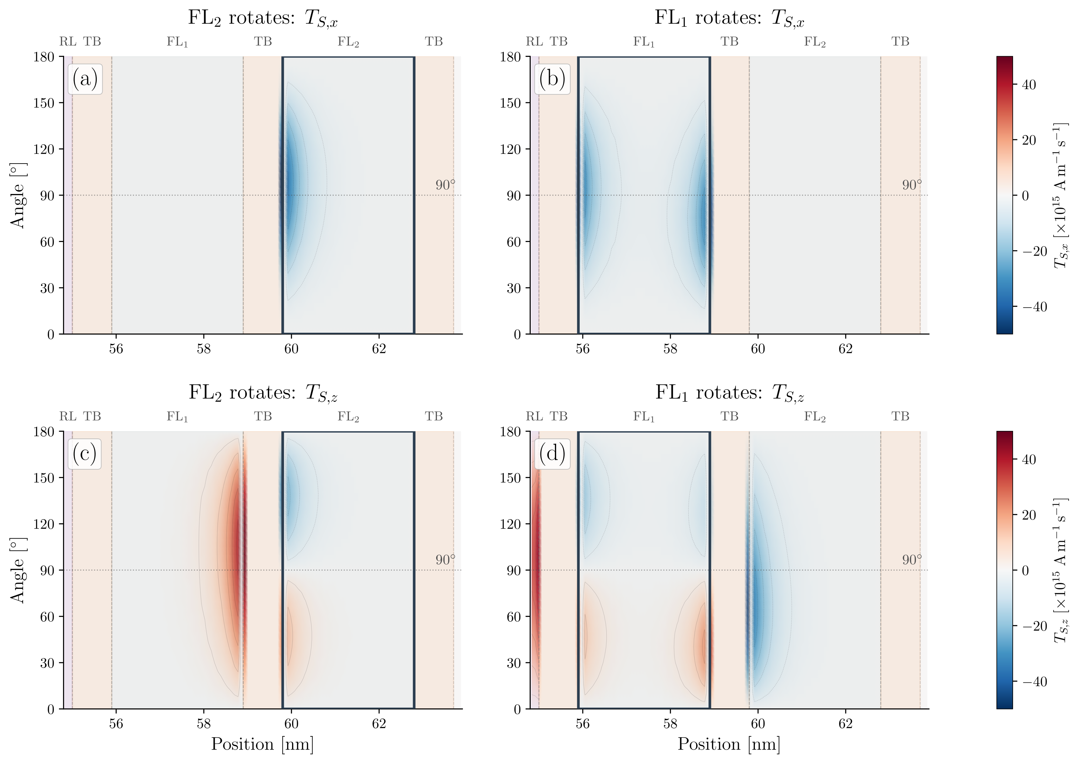
Figure 7.11: Spin-transfer torque heatmap showing \(T_{S,x}\) (top) and \(T_{S,z}\) (bottom) as a function of stack position and magnetization angle for standard polarization (\(P_1 = 0.62\), \(P_2 = 0.57\), \(P_3 = 0.2\)). Left column: FL\(_2\) rotation, right column: FL\(_1\) rotation. Contour lines indicate torque magnitude within ferromagnetic layers.
7.4.1.2 P\(\to \)AP: Competing Torques and Back-Hopping Origin

In the initial P configuration (\(\mathbf {m}_1 = \mathbf {m}_2 = +\hat {x}\)), the reversed bias drives the RL torque on FL\(_1\) toward \(-\hat {x}\):

\begin{equation} \mathbf {T}_{1,\text {RL}} \propto -\mathbf {m}_1 \times (\mathbf {m}_1 \times (+\hat {x})) \label {eq::T1-RL-P} \end{equation}

However, the torque from FL\(_2\) through TB\(_2\) opposes this reversal:

\begin{equation} \mathbf {T}_{1,\text {FL}_2} \propto \mathbf {m}_1 \times (\mathbf {m}_1 \times (+\hat {x})) \label {eq::T1-FL2-P} \end{equation}

These torques partially cancel on FL\(_1\), while the torque on FL\(_2\) from FL\(_1\), given by:

\begin{equation} \mathbf {T}_{2,\text {FL}_1} \propto -\mathbf {m}_2 \times (\mathbf {m}_2 \times (+\hat {x})) \label {eq::T2-FL1-P} \end{equation}

drives FL\(_2\) toward \(-\hat {x}\) unopposed. After FL\(_2\) reverses, both torques on FL\(_1\) become cooperative:

\begin{equation} \mathbf {T}_{1,\text {RL}} + \mathbf {T}_{1,\text {FL}_2} \propto -\mathbf {m}_1 \times (\mathbf {m}_1 \times (+\hat {x})) + \mathbf {m}_1 \times (\mathbf {m}_1 \times (-\hat {x})) \label {eq::T1-combined-P} \end{equation}

Both terms drive FL\(_1\) toward \(-\hat {x}\), producing a slow first phase (opposing torques) followed by a fast second phase (cooperative torques). After both segments reach the AP state (\(\mathbf {m}_1 = \mathbf {m}_2 = -\hat {x}\)), the torque landscape reconfigures. Substituting \(\mathbf {m}_1 = -\hat {x}\) into (7.9):

\begin{equation} \mathbf {T}_{2,\text {FL}_1} \propto -\mathbf {m}_2 \times (\mathbf {m}_2 \times (-\hat {x})) = \mathbf {m}_2 \times (\mathbf {m}_2 \times (+\hat {x})) \label {eq::T2-FL1-backhop} \end{equation}

(image)

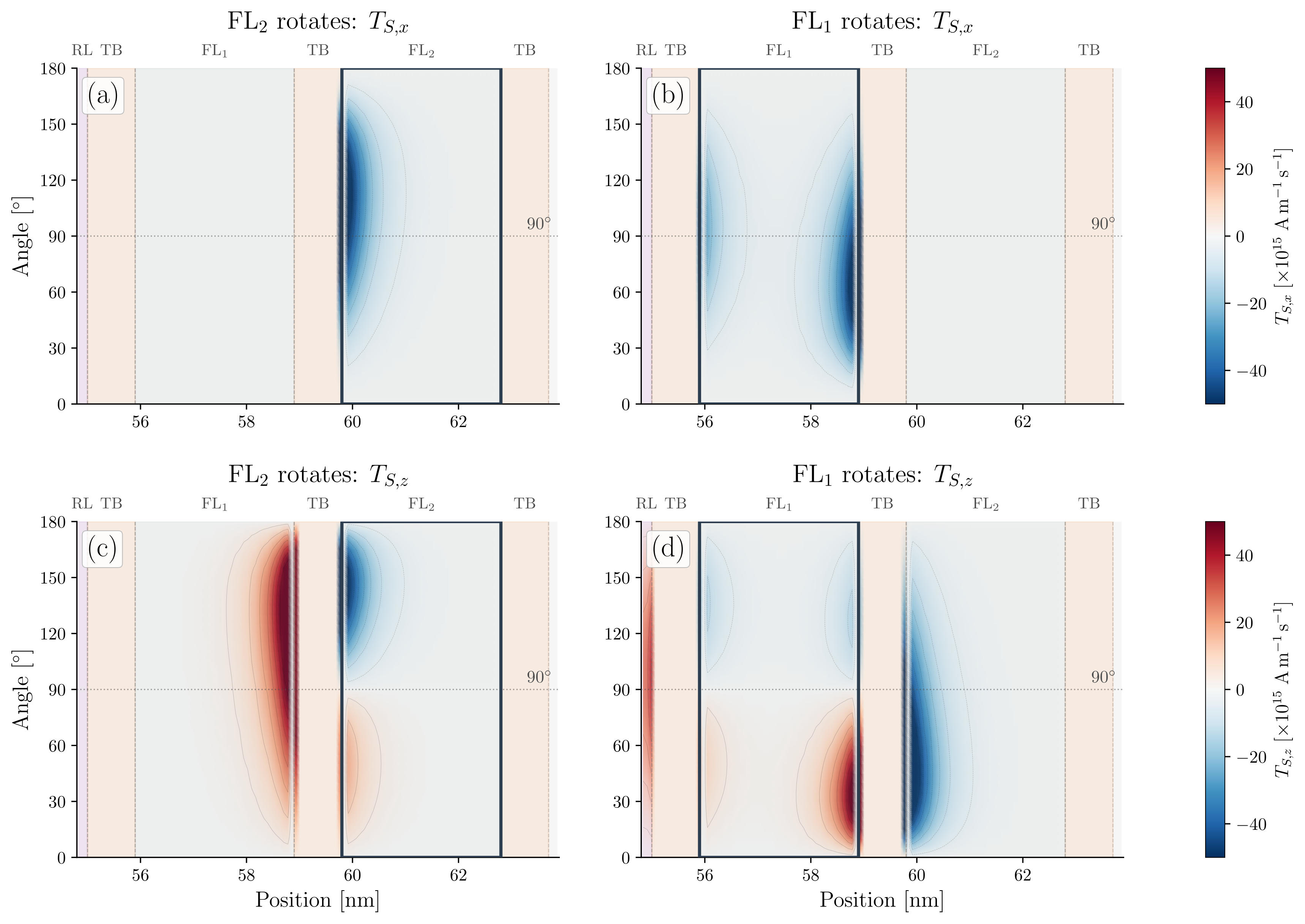
Figure 7.12: Spin-transfer torque heatmap for enhanced TB\(_2\) polarization (\(P_1 = 0.5\), \(P_2 = 0.9\), \(P_3 = 0.2\)). Same layout as Figure 7.11. The enhanced polarization introduces a pronounced torque imbalance: \(T_{S,x}\) on FL\(_1\) is significantly enhanced by the high \(P_2 = 0.9\), while the torque on FL\(_2\) is reduced by the lower \(P_3 = 0.2\).

This torque drives \(\mathbf {m}_2\) toward \(+\hat {x}\) (the initial P orientation) rather than stabilizing the AP state, triggering back-hopping when (7.1) is satisfied.

After FL\(_2\) backhops to \(+\hat {x}\) (while FL\(_1\) remains at \(-\hat {x}\)), the torque on FL\(_1\) from FL\(_2\) through TB\(_2\) becomes:

\begin{equation} \mathbf {T}_{1,\text {FL}_2} \propto \mathbf {m}_1 \times (\mathbf {m}_1 \times (+\hat {x})) \label {eq::T1-FL2-backhop} \end{equation}

driving \(\mathbf {m}_1\) toward \(+\hat {x}\), while the RL torque through TB\(_1\) opposes:

\begin{equation} \mathbf {T}_{1,\text {RL}} \propto -\mathbf {m}_1 \times (\mathbf {m}_1 \times (+\hat {x})) \label {eq::T1-RL-backhop} \end{equation}

The net torque on FL\(_1\), with magnitudes scaling as \(P_2\) and \(P_1\):

\begin{equation} \mathbf {T}_1 \propto (P_2 - P_1)\,\mathbf {m}_1 \times (\mathbf {m}_1 \times (+\hat {x})) \label {eq::T1-net-backhop} \end{equation}

(image)

Figure 7.13: Three-dimensional surface representation of \(T_{S,x}\) (a, b) and \(T_{S,z}\) (c, d) for standard polarization (\(P_1 = 0.62\), \(P_2 = 0.57\), \(P_3 = 0.2\)). Panels (a, c): FL\(_2\) rotation, (b, d): FL\(_1\) rotation. The in-plane torque \(T_{S,x}\) is negative throughout the angular range with a minimum near \(90^\circ \). A Gaussian filter suppresses numerical noise from the FE mesh.

For \(P_2 = 0.9 > P_1 = 0.5\), the FL\(_2\) torque dominates, driving FL\(_1\) back to \(+\hat {x}\) and completing the cycle. The time-resolved data (Figure 7.15) confirms a \(10\times \) TB\(_2\) torque surge at back-hopping onset.

The heatmaps are constructed by systematically sampling the torque landscape of the composite FL. For each configuration, one FL segment is held at a fixed orientation. At the same time, the other is rotated in the \(xz\)-plane (about \(\hat {y}\)) in \(5^\circ \) increments from the parallel (\(0^\circ \)) to the anti-parallel (\(180^\circ \)) alignment. Specifically, for the P\(\to \)AP-relevant landscape: FL\(_1\) is fixed in the P orientation (\(+\hat {x}\)) while FL\(_2\) is rotated from P (\(0^\circ \)) toward AP (\(180^\circ \)). Subsequently, FL\(_2\) is fixed in the P orientation, and FL\(_1\) is rotated from AP (\(180^\circ \)) toward P (\(0^\circ \)). At each angular step, the coupled spin-transport equations are solved self-consistently to obtain the full spatial torque distribution. This procedure maps the torque experienced by each segment as a function of the other’s orientation, capturing the non-additive inter-segment coupling.

(image)

Figure 7.14: Three-dimensional torque surfaces for enhanced TB\(_2\) polarization (\(P_1 = 0.5\), \(P_2 = 0.9\), \(P_3 = 0.2\)). Compared to the standard case (Figure 7.13), \(T_{S,x}\) on FL\(_1\) (b) reaches approximately twice the magnitude of FL\(_2\) (a), reflecting the \(P_2/P_3 = 0.9/0.2\) ratio. This imbalance drives sequential switching and back-hopping.

The resulting heatmaps quantify the torque imbalance: in the standard case (Figure 7.11), \(T_{S,x}\) peaks at comparable magnitudes (\({\sim }{-}20 \times 10^{15}\) A/(m s)) for both FL segments, while the enhanced configuration (Figure 7.12) doubles this to \({\sim }{-}40 \times 10^{15}\) A/(m s) for FL\(_1\), reflecting \(P_2/P_3 = 0.9/0.2\). The perpendicular torque \(T_{S,z}\) intensifies at TB\(_2\) with a sign change near \(90^\circ \), creating the destabilizing field responsible for back-hopping.

The three-dimensional surfaces (Figure 7.13, Figure 7.14) confirm the \(2\times \) amplification across both torque components, with the \(T_{S,x}\) angular profile exhibiting a clear \(\sin (\theta )\) dependence characteristic of the drift-diffusion mechanism, ruling out numerical artifacts.

These spatial torque data provide an explanation for the directional asymmetry: during P\(\to \)AP, the \(T_{S,z}\) sign change near \(90^\circ \) at the TB\(_2\) interface (Figure 7.12) constitutes the destabilizing field that, when the instability condition (7.1) is satisfied, triggers the back-hopping cascade established in Section 7.4. During AP\(\to \)P, both TB\(_1\) and TB\(_2\) torques cooperate to stabilize the final P state, and the torques vanish smoothly at \(\theta \to 0^\circ \) without sign reversal. The slower initial P\(\to \)AP phase arises because the flux-closure stray field from both FL segments at \(+\hat {x}\) opposes the initial torque, whereas AP\(\to \)P benefits from stray field assistance. This framework also explains the voltage-polarity asymmetry (Section 7.4.5): the cooperative torque configuration renders the P state immune to wrong-polarity switching, whereas the AP state becomes unstable above \(\SI {3.0}{\volt }\).

(image)

Figure 7.15: Decomposition of damping-like and field-like spin-transfer torques on FL\(_1\) and FL\(_2\) during (a) AP\(\to \)P and (b) P\(\to \)AP switching. The torque hierarchy between TB\(_1\) and TB\(_2\) governs the sequential switching order and determines back-hopping onset  [199].

The TB\(_1\) torque (initial magnitude \({\sim }5 \times 10^{15}\) A/(m s)) initiates the first segment reversal in each direction. During AP\(\to \)P (Figure 7.15 (a)), the reconfigured TB\(_2\) torque on FL\(_2\) reaches \(T_{S,z} \sim {+}4 \times 10^{15}\) A/(m s), cooperating with TB\(_1\) for a smooth transition. During P\(\to \)AP (Figure 7.15 (b)), the TB\(_2\) torque surges to \(T_{S,z} \sim {+}40 \times 10^{15}\) A/(m s) after both segments reach the AP state, a \(10\times \) asymmetry that quantitatively explains why only P\(\to \)AP satisfies the instability condition (7.1). The field-like torque \(T_{S,x}\) remains comparatively small, modifying the precession trajectory without altering the switching sequence  [200].

The combined trajectory and torque data confirm three key properties: (1) the oscillation period scales with FL segment length, establishing back-hopping as deterministic, (2) shorter segments (2nm to 3nm) exhibit more pronounced cycling due to lower anisotropy barriers, and (3) the \(2\times \) torque amplification from \(P_2 = 0.57\) to \(0.9\) (Figure 7.11–Figure 7.14) provides a quantitative design knob for back-hopping control.

7.4.2 Cyclic Switching Visualization

(image)

Figure 7.16: Cyclic switching visualization during P\(\to \)AP transition: three-dimensional magnetization snapshots at five characteristic stages (i)–(vi) of the FL reversal cycle, colored by the \(m_x\) magnetization component. Based on  [199].

Figure 7.16 visualizes the complete P\(\to \)AP back-hopping cycle through three-dimensional magnetization snapshots. The five stages trace the trajectory through all four composite FL states: (i) initial P (\(\to \,\to \,\to \), State 1), (ii) FL\(_2\) reversal (\(\to \,\to \,\leftarrow \), State 2), (iii) cooperative FL\(_1\) switching, full AP (\(\to \,\leftarrow \,\leftarrow \), State 3), (iv) FL\(_2\) back-hopping (7.11) (\(\to \,\leftarrow \,\to \), State 4), and (v) FL\(_1\) return (7.14) to State 1. The critical transition (iv)\(\to \)(v) occurs when \(T_{S,z}\) at the TB\(_2\) interface increases by approximately one order of magnitude (Figure 7.12), crossing the instability threshold (7.1).

7.4.3 Multi-Level Cell Realization

The deterministic cyclic switching enables multi-level cell operation: a composite FL with controlled back-hopping supports four distinct magnetization states  [193], summarized in Table 7.3.

Table 7.3: Multi-level cell state definitions and characteristics.
.
State FL\(_1\) vs. RL FL\(_2\) vs. RL Overall Resistance Binary Code
1 Parallel Parallel Lowest 00
2 Parallel Anti-parallel Low-Medium 01
3 Anti-parallel Anti-parallel Highest 11
4 Anti-parallel Parallel Medium-High 10

(image)

Figure 7.17: Resistance (purple, left axis) and average magnetization \(m_x\) (orange dashed, right axis) as a function of time for four pulse durations: (a) \(t_\mathrm {pulse} = \SI {1.0}{\nano \second }\), (b) 1.3ns, (c) 2.0ns, and (d) 3.0ns. The vertical dotted line marks pulse termination \(t_\mathrm {off}\). The four resistance levels are clearly distinguishable with \({>}20\%\) separation between adjacent states. Based on Figure  [194].

The cyclic P\(\to \)AP trajectory traverses all four states (\(1 \to 2 \to 3 \to 4 \to 1 \to \ldots \)), visiting four unique resistance levels per cycle and validating four-level MLC operation. By controlling the write pulse duration, any state can be accessed and stabilized when the bias is removed.

Figure 7.17 confirms \(>\)20% resistance separation between adjacent states, stable retention after pulse removal, and reproducibility over multiple cycles. Pulse duration precision of approximately 100ps is required.

7.4.4 FL Thickness Variation

Since FL thickness controls the anisotropy barrier and back-hopping onset, the pulse duration dependence is examined for the 3nm symmetric structure to establish the MLC operational window.

Figure 7.18 maps the pulse-duration operational window for the 3nm symmetric structure. Short pulses (\(t_\mathrm {pulse} \lesssim \SI {0.8}{\nano \second }\), red curves) return the magnetization to the initial state. Intermediate durations (1ns to 2ns) access distinct partial-switching configurations, and the longest pulses (\(t_\mathrm {pulse} > \SI {2.5}{\nano \second }\), dark blue) drive a full back-hopping cycle, confirming the cyclic trajectory of Section 7.4.2. The FL length dependence of the stable-state window was established in Section 7.3.5.

7.4.5 Voltage Polarity Robustness

Figure 7.19 shows the magnetization response under reversed voltage polarity (opposite to the polarity required for switching) for both initial states.

(image)

Figure 7.18: Average magnetization \(\langle m_x \rangle \) versus time for P\(\to \)AP switching at 1.5V bias with write pulse durations ranging from 0 to 3.5ns (color-coded from red for short pulses to blue for long pulses). By terminating the write pulse at different times, distinct final magnetization configurations are accessed: short pulses (\(t_\mathrm {pulse} \lesssim \SI {0.8}{\nano \second }\)) return the composite FL to its initial state, intermediate pulses stabilize partial-switching configurations, and the longest pulses (\(t_\mathrm {pulse} > \SI {2.5}{\nano \second }\)) drive a complete back-hopping cycle. Based on  [199].

(image)

Figure 7.19: Magnetization response under reversed voltage polarity (opposite to the polarity required for switching): (a) AP state with positive voltage, stable at \(m_x \approx -1\) for \(V \leq \SI {2.5}{\volt }\), but cyclic oscillations between \(m_x = -1\) and \(+1\) emerge at \(V \geq \SI {3.0}{\volt }\) with increasing frequency, (b) P state with negative voltage, stable at \(m_x = +1\) across the entire range (2.0V to 4.5V). The asymmetry arises from the cooperative torque configuration of the P state: both TB\(_1\) and TB\(_2\) torques act to stabilize the parallel alignment (see Section 7.4.1), whereas the AP state suffers from competing torques that enable destabilization at sufficient voltage.

The P state is immune to reversed-polarity torques across the entire voltage range: the cooperative torque configuration (both TB\(_1\) and TB\(_2\) torques stabilize the parallel alignment, cf. Section 7.4.1) prevents destabilization regardless of voltage magnitude. In contrast, the AP state, characterized by competing torques between TB\(_1\) and TB\(_2\), becomes unstable above a voltage threshold where the net torque overcomes the anisotropy barrier and initiates cyclic back-hopping. This asymmetry follows directly from the torque hierarchy established in Section 7.4.1 and confirms back-hopping as a deterministic torque-driven phenomenon  [200].

New physical insight. Back-hopping in composite FL structures is a deterministic, torque-hierarchy-driven phenomenon robust across material parameter sets, not the stochastic thermal effect assumed in prior literature  [188, 195, 201]. The cyclic dynamics are controllable through TB\(_2\) polarization and FL segment length, enabling four-state MLC operation with distinct resistance levels addressable via pulse duration modulation at 100ps resolution  [193, 194], transforming a write error into a \(4\times \) storage density increase.