[ Previous ] [ Home ] [ Next ]

Numerical Analysis and Innovative Simulation
Techniques for Designing Advanced MRAM

\(\newcommand{\footnotename}{footnote}\) \(\def \LWRfootnote {1}\) \(\newcommand {\footnote }[2][\LWRfootnote ]{{}^{\mathrm {#1}}}\) \(\newcommand {\footnotemark }[1][\LWRfootnote ]{{}^{\mathrm {#1}}}\) \(\let \LWRorighspace \hspace \) \(\renewcommand {\hspace }{\ifstar \LWRorighspace \LWRorighspace }\) \(\newcommand {\TextOrMath }[2]{#2}\) \(\newcommand {\mathnormal }[1]{{#1}}\) \(\newcommand \ensuremath [1]{#1}\) \(\newcommand {\LWRframebox }[2][]{\fbox {#2}} \newcommand {\framebox }[1][]{\LWRframebox } \) \(\newcommand {\setlength }[2]{}\) \(\newcommand {\addtolength }[2]{}\) \(\newcommand {\setcounter }[2]{}\) \(\newcommand {\addtocounter }[2]{}\) \(\newcommand {\arabic }[1]{}\) \(\newcommand {\number }[1]{}\) \(\newcommand {\noalign }[1]{\text {#1}\notag \\}\) \(\newcommand {\cline }[1]{}\) \(\newcommand {\directlua }[1]{\text {(directlua)}}\) \(\newcommand {\luatexdirectlua }[1]{\text {(directlua)}}\) \(\newcommand {\protect }{}\) \(\def \LWRabsorbnumber #1 {}\) \(\def \LWRabsorbquotenumber "#1 {}\) \(\newcommand {\LWRabsorboption }[1][]{}\) \(\newcommand {\LWRabsorbtwooptions }[1][]{\LWRabsorboption }\) \(\def \mathchar {\ifnextchar "\LWRabsorbquotenumber \LWRabsorbnumber }\) \(\def \mathcode #1={\mathchar }\) \(\let \delcode \mathcode \) \(\let \delimiter \mathchar \) \(\def \oe {\unicode {x0153}}\) \(\def \OE {\unicode {x0152}}\) \(\def \ae {\unicode {x00E6}}\) \(\def \AE {\unicode {x00C6}}\) \(\def \aa {\unicode {x00E5}}\) \(\def \AA {\unicode {x00C5}}\) \(\def \o {\unicode {x00F8}}\) \(\def \O {\unicode {x00D8}}\) \(\def \l {\unicode {x0142}}\) \(\def \L {\unicode {x0141}}\) \(\def \ss {\unicode {x00DF}}\) \(\def \SS {\unicode {x1E9E}}\) \(\def \dag {\unicode {x2020}}\) \(\def \ddag {\unicode {x2021}}\) \(\def \P {\unicode {x00B6}}\) \(\def \copyright {\unicode {x00A9}}\) \(\def \pounds {\unicode {x00A3}}\) \(\let \LWRref \ref \) \(\renewcommand {\ref }{\ifstar \LWRref \LWRref }\) \( \newcommand {\multicolumn }[3]{#3}\) \(\require {textcomp}\) \(\newcommand {\mathlarger }[1]{#1}\) \(\newcommand {\mathsmaller }[1]{#1}\) \(\newcommand {\intertext }[1]{\text {#1}\notag \\}\) \(\let \Hat \hat \) \(\let \Check \check \) \(\let \Tilde \tilde \) \(\let \Acute \acute \) \(\let \Grave \grave \) \(\let \Dot \dot \) \(\let \Ddot \ddot \) \(\let \Breve \breve \) \(\let \Bar \bar \) \(\let \Vec \vec \) \(\newcommand {\toprule }[1][]{\hline }\) \(\let \midrule \toprule \) \(\let \bottomrule \toprule \) \(\def \LWRbooktabscmidruleparen (#1)#2{}\) \(\newcommand {\LWRbooktabscmidrulenoparen }[1]{}\) \(\newcommand {\cmidrule }[1][]{\ifnextchar (\LWRbooktabscmidruleparen \LWRbooktabscmidrulenoparen }\) \(\newcommand {\morecmidrules }{}\) \(\newcommand {\specialrule }[3]{\hline }\) \(\newcommand {\addlinespace }[1][]{}\) \(\newcommand {\bm }[1]{\boldsymbol {#1}}\) \(\newcommand {\LWRsubmultirow }[2][]{#2}\) \(\newcommand {\LWRmultirow }[2][]{\LWRsubmultirow }\) \(\newcommand {\multirow }[2][]{\LWRmultirow }\) \(\newcommand {\mrowcell }{}\) \(\newcommand {\mcolrowcell }{}\) \(\newcommand {\STneed }[1]{}\) \(\newcommand {\tothe }[1]{^{#1}}\) \(\newcommand {\raiseto }[2]{{#2}^{#1}}\) \(\newcommand {\LWRsiunitxEND }{}\) \(\def \LWRsiunitxang #1;#2;#3;#4\LWRsiunitxEND {\ifblank {#1}{}{\num {#1}\degree }\ifblank {#2}{}{\num {#2}^{\unicode {x2032}}}\ifblank {#3}{}{\num {#3}^{\unicode {x2033}}}}\) \(\newcommand {\ang }[2][]{\LWRsiunitxang #2;;;\LWRsiunitxEND }\) \(\def \LWRsiunitxdistribunit {}\) \(\newcommand {\LWRsiunitxENDTWO }{}\) \(\def \LWRsiunitxprintdecimalsubtwo #1,#2,#3\LWRsiunitxENDTWO {\ifblank {#1}{0}{\mathrm {#1}}\ifblank {#2}{}{{\LWRsiunitxdecimal }\mathrm {#2}}}\) \(\def \LWRsiunitxprintdecimalsub #1.#2.#3\LWRsiunitxEND {\LWRsiunitxprintdecimalsubtwo #1,,\LWRsiunitxENDTWO \ifblank {#2}{}{{\LWRsiunitxdecimal }\LWRsiunitxprintdecimalsubtwo #2,,\LWRsiunitxENDTWO }}\) \(\newcommand {\LWRsiunitxprintdecimal }[1]{\LWRsiunitxprintdecimalsub #1...\LWRsiunitxEND }\) \(\def \LWRsiunitxnumplus #1+#2+#3\LWRsiunitxEND {\ifblank {#2}{\LWRsiunitxprintdecimal {#1}}{\ifblank {#1}{\LWRsiunitxprintdecimal {#2}}{\LWRsiunitxprintdecimal {#1}\unicode {x02B}\LWRsiunitxprintdecimal {#2}}}\LWRsiunitxdistribunit }\) \(\def \LWRsiunitxnumminus #1-#2-#3\LWRsiunitxEND {\ifblank {#2}{\LWRsiunitxnumplus #1+++\LWRsiunitxEND }{\ifblank {#1}{}{\LWRsiunitxprintdecimal {#1}}\unicode {x02212}\LWRsiunitxprintdecimal {#2}\LWRsiunitxdistribunit }}\) \(\def \LWRsiunitxnumpmmacro #1\pm #2\pm #3\LWRsiunitxEND {\ifblank {#2}{\LWRsiunitxnumminus #1---\LWRsiunitxEND }{\LWRsiunitxprintdecimal {#1}\unicode {x0B1}\LWRsiunitxprintdecimal {#2}\LWRsiunitxdistribunit }}\) \(\def \LWRsiunitxnumpm #1+-#2+-#3\LWRsiunitxEND {\ifblank {#2}{\LWRsiunitxnumpmmacro #1\pm \pm \pm \LWRsiunitxEND }{\LWRsiunitxprintdecimal {#1}\unicode {x0B1}\LWRsiunitxprintdecimal {#2}\LWRsiunitxdistribunit }}\) \(\newcommand {\LWRsiunitxnumscientific }[2]{\ifblank {#1}{}{\ifstrequal {#1}{-}{-}{\LWRsiunitxprintdecimal {#1}\times }}10^{\LWRsiunitxprintdecimal {#2}}\LWRsiunitxdistribunit }\) \(\def \LWRsiunitxnumD #1D#2D#3\LWRsiunitxEND {\ifblank {#2}{\LWRsiunitxnumpm #1+-+-\LWRsiunitxEND }{\mathrm {\LWRsiunitxnumscientific {#1}{#2}}}}\) \(\def \LWRsiunitxnumd #1d#2d#3\LWRsiunitxEND {\ifblank {#2}{\LWRsiunitxnumD #1DDD\LWRsiunitxEND }{\mathrm {\LWRsiunitxnumscientific {#1}{#2}}}}\) \(\def \LWRsiunitxnumE #1E#2E#3\LWRsiunitxEND {\ifblank {#2}{\LWRsiunitxnumd #1ddd\LWRsiunitxEND }{\mathrm {\LWRsiunitxnumscientific {#1}{#2}}}}\) \(\def \LWRsiunitxnume #1e#2e#3\LWRsiunitxEND {\ifblank {#2}{\LWRsiunitxnumE #1EEE\LWRsiunitxEND }{\mathrm {\LWRsiunitxnumscientific {#1}{#2}}}}\) \(\def \LWRsiunitxnumx #1x#2x#3x#4\LWRsiunitxEND {\ifblank {#2}{\LWRsiunitxnume #1eee\LWRsiunitxEND }{\ifblank {#3}{\LWRsiunitxnume #1eee\LWRsiunitxEND \times \LWRsiunitxnume #2eee\LWRsiunitxEND }{\LWRsiunitxnume #1eee\LWRsiunitxEND \times \LWRsiunitxnume #2eee\LWRsiunitxEND \times \LWRsiunitxnume #3eee\LWRsiunitxEND }}}\) \(\newcommand {\num }[2][]{\LWRsiunitxnumx #2xxxxx\LWRsiunitxEND }\) \(\newcommand {\si }[2][]{\mathrm {\gsubstitute {#2}{~}{\,}}}\) \(\def \LWRsiunitxSIopt #1[#2]#3{\def \LWRsiunitxdistribunit {\,\si {#3}}{#2}\num {#1}\def \LWRsiunitxdistribunit {}}\) \(\newcommand {\LWRsiunitxSI }[2]{\def \LWRsiunitxdistribunit {\,\si {#2}}\num {#1}\def \LWRsiunitxdistribunit {}}\) \(\newcommand {\SI }[2][]{\ifnextchar [{\LWRsiunitxSIopt {#2}}{\LWRsiunitxSI {#2}}}\) \(\newcommand {\numlist }[2][]{\text {#2}}\) \(\newcommand {\numrange }[3][]{\num {#2}\ \LWRsiunitxrangephrase \ \num {#3}}\) \(\newcommand {\SIlist }[3][]{\text {#2}\,\si {#3}}\) \(\newcommand {\SIrange }[4][]{\num {#2}\,#4\ \LWRsiunitxrangephrase \ \num {#3}\,#4}\) \(\newcommand {\tablenum }[2][]{\mathrm {#2}}\) \(\newcommand {\ampere }{\mathrm {A}}\) \(\newcommand {\candela }{\mathrm {cd}}\) \(\newcommand {\kelvin }{\mathrm {K}}\) \(\newcommand {\kilogram }{\mathrm {kg}}\) \(\newcommand {\metre }{\mathrm {m}}\) \(\newcommand {\mole }{\mathrm {mol}}\) \(\newcommand {\second }{\mathrm {s}}\) \(\newcommand {\becquerel }{\mathrm {Bq}}\) \(\newcommand {\degreeCelsius }{\unicode {x2103}}\) \(\newcommand {\coulomb }{\mathrm {C}}\) \(\newcommand {\farad }{\mathrm {F}}\) \(\newcommand {\gray }{\mathrm {Gy}}\) \(\newcommand {\hertz }{\mathrm {Hz}}\) \(\newcommand {\henry }{\mathrm {H}}\) \(\newcommand {\joule }{\mathrm {J}}\) \(\newcommand {\katal }{\mathrm {kat}}\) \(\newcommand {\lumen }{\mathrm {lm}}\) \(\newcommand {\lux }{\mathrm {lx}}\) \(\newcommand {\newton }{\mathrm {N}}\) \(\newcommand {\ohm }{\mathrm {\Omega }}\) \(\newcommand {\pascal }{\mathrm {Pa}}\) \(\newcommand {\radian }{\mathrm {rad}}\) \(\newcommand {\siemens }{\mathrm {S}}\) \(\newcommand {\sievert }{\mathrm {Sv}}\) \(\newcommand {\steradian }{\mathrm {sr}}\) \(\newcommand {\tesla }{\mathrm {T}}\) \(\newcommand {\volt }{\mathrm {V}}\) \(\newcommand {\watt }{\mathrm {W}}\) \(\newcommand {\weber }{\mathrm {Wb}}\) \(\newcommand {\day }{\mathrm {d}}\) \(\newcommand {\degree }{\mathrm {^\circ }}\) \(\newcommand {\hectare }{\mathrm {ha}}\) \(\newcommand {\hour }{\mathrm {h}}\) \(\newcommand {\litre }{\mathrm {l}}\) \(\newcommand {\liter }{\mathrm {L}}\) \(\newcommand {\arcminute }{^\prime }\) \(\newcommand {\minute }{\mathrm {min}}\) \(\newcommand {\arcsecond }{^{\prime \prime }}\) \(\newcommand {\tonne }{\mathrm {t}}\) \(\newcommand {\astronomicalunit }{au}\) \(\newcommand {\atomicmassunit }{u}\) \(\newcommand {\bohr }{\mathit {a}_0}\) \(\newcommand {\clight }{\mathit {c}_0}\) \(\newcommand {\dalton }{\mathrm {D}_\mathrm {a}}\) \(\newcommand {\electronmass }{\mathit {m}_{\mathrm {e}}}\) \(\newcommand {\electronvolt }{\mathrm {eV}}\) \(\newcommand {\elementarycharge }{\mathit {e}}\) \(\newcommand {\hartree }{\mathit {E}_{\mathrm {h}}}\) \(\newcommand {\planckbar }{\mathit {\unicode {x210F}}}\) \(\newcommand {\angstrom }{\mathrm {\unicode {x212B}}}\) \(\let \LWRorigbar \bar \) \(\newcommand {\bar }{\mathrm {bar}}\) \(\newcommand {\barn }{\mathrm {b}}\) \(\newcommand {\bel }{\mathrm {B}}\) \(\newcommand {\decibel }{\mathrm {dB}}\) \(\newcommand {\knot }{\mathrm {kn}}\) \(\newcommand {\mmHg }{\mathrm {mmHg}}\) \(\newcommand {\nauticalmile }{\mathrm {M}}\) \(\newcommand {\neper }{\mathrm {Np}}\) \(\newcommand {\yocto }{\mathrm {y}}\) \(\newcommand {\zepto }{\mathrm {z}}\) \(\newcommand {\atto }{\mathrm {a}}\) \(\newcommand {\femto }{\mathrm {f}}\) \(\newcommand {\pico }{\mathrm {p}}\) \(\newcommand {\nano }{\mathrm {n}}\) \(\newcommand {\micro }{\mathrm {\unicode {x00B5}}}\) \(\newcommand {\milli }{\mathrm {m}}\) \(\newcommand {\centi }{\mathrm {c}}\) \(\newcommand {\deci }{\mathrm {d}}\) \(\newcommand {\deca }{\mathrm {da}}\) \(\newcommand {\hecto }{\mathrm {h}}\) \(\newcommand {\kilo }{\mathrm {k}}\) \(\newcommand {\mega }{\mathrm {M}}\) \(\newcommand {\giga }{\mathrm {G}}\) \(\newcommand {\tera }{\mathrm {T}}\) \(\newcommand {\peta }{\mathrm {P}}\) \(\newcommand {\exa }{\mathrm {E}}\) \(\newcommand {\zetta }{\mathrm {Z}}\) \(\newcommand {\yotta }{\mathrm {Y}}\) \(\newcommand {\percent }{\mathrm {\%}}\) \(\newcommand {\meter }{\mathrm {m}}\) \(\newcommand {\metre }{\mathrm {m}}\) \(\newcommand {\gram }{\mathrm {g}}\) \(\newcommand {\kg }{\kilo \gram }\) \(\newcommand {\of }[1]{_{\mathrm {#1}}}\) \(\newcommand {\squared }{^2}\) \(\newcommand {\square }[1]{\mathrm {#1}^2}\) \(\newcommand {\cubed }{^3}\) \(\newcommand {\cubic }[1]{\mathrm {#1}^3}\) \(\newcommand {\per }{\,\mathrm {/}}\) \(\newcommand {\celsius }{\unicode {x2103}}\) \(\newcommand {\fg }{\femto \gram }\) \(\newcommand {\pg }{\pico \gram }\) \(\newcommand {\ng }{\nano \gram }\) \(\newcommand {\ug }{\micro \gram }\) \(\newcommand {\mg }{\milli \gram }\) \(\newcommand {\g }{\gram }\) \(\newcommand {\kg }{\kilo \gram }\) \(\newcommand {\amu }{\mathrm {u}}\) \(\newcommand {\pm }{\pico \metre }\) \(\newcommand {\nm }{\nano \metre }\) \(\newcommand {\um }{\micro \metre }\) \(\newcommand {\mm }{\milli \metre }\) \(\newcommand {\cm }{\centi \metre }\) \(\newcommand {\dm }{\deci \metre }\) \(\newcommand {\m }{\metre }\) \(\newcommand {\km }{\kilo \metre }\) \(\newcommand {\as }{\atto \second }\) \(\newcommand {\fs }{\femto \second }\) \(\newcommand {\ps }{\pico \second }\) \(\newcommand {\ns }{\nano \second }\) \(\newcommand {\us }{\micro \second }\) \(\newcommand {\ms }{\milli \second }\) \(\newcommand {\s }{\second }\) \(\newcommand {\fmol }{\femto \mol }\) \(\newcommand {\pmol }{\pico \mol }\) \(\newcommand {\nmol }{\nano \mol }\) \(\newcommand {\umol }{\micro \mol }\) \(\newcommand {\mmol }{\milli \mol }\) \(\newcommand {\mol }{\mol }\) \(\newcommand {\kmol }{\kilo \mol }\) \(\newcommand {\pA }{\pico \ampere }\) \(\newcommand {\nA }{\nano \ampere }\) \(\newcommand {\uA }{\micro \ampere }\) \(\newcommand {\mA }{\milli \ampere }\) \(\newcommand {\A }{\ampere }\) \(\newcommand {\kA }{\kilo \ampere }\) \(\newcommand {\ul }{\micro \litre }\) \(\newcommand {\ml }{\milli \litre }\) \(\newcommand {\l }{\litre }\) \(\newcommand {\hl }{\hecto \litre }\) \(\newcommand {\uL }{\micro \liter }\) \(\newcommand {\mL }{\milli \liter }\) \(\newcommand {\L }{\liter }\) \(\newcommand {\hL }{\hecto \liter }\) \(\newcommand {\mHz }{\milli \hertz }\) \(\newcommand {\Hz }{\hertz }\) \(\newcommand {\kHz }{\kilo \hertz }\) \(\newcommand {\MHz }{\mega \hertz }\) \(\newcommand {\GHz }{\giga \hertz }\) \(\newcommand {\THz }{\tera \hertz }\) \(\newcommand {\mN }{\milli \newton }\) \(\newcommand {\N }{\newton }\) \(\newcommand {\kN }{\kilo \newton }\) \(\newcommand {\MN }{\mega \newton }\) \(\newcommand {\Pa }{\pascal }\) \(\newcommand {\kPa }{\kilo \pascal }\) \(\newcommand {\MPa }{\mega \pascal }\) \(\newcommand {\GPa }{\giga \pascal }\) \(\newcommand {\mohm }{\milli \ohm }\) \(\newcommand {\kohm }{\kilo \ohm }\) \(\newcommand {\Mohm }{\mega \ohm }\) \(\newcommand {\pV }{\pico \volt }\) \(\newcommand {\nV }{\nano \volt }\) \(\newcommand {\uV }{\micro \volt }\) \(\newcommand {\mV }{\milli \volt }\) \(\newcommand {\V }{\volt }\) \(\newcommand {\kV }{\kilo \volt }\) \(\newcommand {\W }{\watt }\) \(\newcommand {\uW }{\micro \watt }\) \(\newcommand {\mW }{\milli \watt }\) \(\newcommand {\kW }{\kilo \watt }\) \(\newcommand {\MW }{\mega \watt }\) \(\newcommand {\GW }{\giga \watt }\) \(\newcommand {\J }{\joule }\) \(\newcommand {\uJ }{\micro \joule }\) \(\newcommand {\mJ }{\milli \joule }\) \(\newcommand {\kJ }{\kilo \joule }\) \(\newcommand {\eV }{\electronvolt }\) \(\newcommand {\meV }{\milli \electronvolt }\) \(\newcommand {\keV }{\kilo \electronvolt }\) \(\newcommand {\MeV }{\mega \electronvolt }\) \(\newcommand {\GeV }{\giga \electronvolt }\) \(\newcommand {\TeV }{\tera \electronvolt }\) \(\newcommand {\kWh }{\kilo \watt \hour }\) \(\newcommand {\F }{\farad }\) \(\newcommand {\fF }{\femto \farad }\) \(\newcommand {\pF }{\pico \farad }\) \(\newcommand {\K }{\mathrm {K}}\) \(\newcommand {\dB }{\mathrm {dB}}\) \(\newcommand {\kibi }{\mathrm {Ki}}\) \(\newcommand {\mebi }{\mathrm {Mi}}\) \(\newcommand {\gibi }{\mathrm {Gi}}\) \(\newcommand {\tebi }{\mathrm {Ti}}\) \(\newcommand {\pebi }{\mathrm {Pi}}\) \(\newcommand {\exbi }{\mathrm {Ei}}\) \(\newcommand {\zebi }{\mathrm {Zi}}\) \(\newcommand {\yobi }{\mathrm {Yi}}\) \(\let \unit \si \) \(\let \qty \SI \) \(\let \qtylist \SIlist \) \(\let \qtyrange \SIrange \) \(\let \numproduct \num \) \(\let \qtyproduct \SI \) \(\let \complexnum \num \) \(\newcommand {\complexqty }[3][]{(\complexnum {#2})\si {#3}}\) \(\require {mathtools}\) \(\newcommand {\vcentcolon }{\mathrel {\unicode {x2236}}}\) \(\newcommand {\approxcolon }{\approx \vcentcolon }\) \(\newcommand {\Approxcolon }{\approx \dblcolon }\) \(\newcommand {\simcolon }{\sim \vcentcolon }\) \(\newcommand {\Simcolon }{\sim \dblcolon }\) \(\newcommand {\dashcolon }{\mathrel {-}\vcentcolon }\) \(\newcommand {\Dashcolon }{\mathrel {-}\dblcolon }\) \(\newcommand {\colondash }{\vcentcolon \mathrel {-}}\) \(\newcommand {\Colondash }{\dblcolon \mathrel {-}}\) \(\newenvironment {crampedsubarray}[1]{}{}\) \(\newcommand {\smashoperator }[2][]{#2\limits }\) \(\newcommand {\SwapAboveDisplaySkip }{}\) \(\newcommand {\LaTeXunderbrace }[1]{\underbrace {#1}}\) \(\newcommand {\LaTeXoverbrace }[1]{\overbrace {#1}}\) \(\Newextarrow \xLongleftarrow {10,10}{0x21D0}\) \(\Newextarrow \xLongrightarrow {10,10}{0x21D2}\) \(\let \xlongleftarrow \xleftarrow \) \(\let \xlongrightarrow \xrightarrow \) \(\newcommand {\LWRmultlined }[1][]{\begin {multline*}}\) \(\newenvironment {multlined}[1][]{\LWRmultlined }{\end {multline*}}\) \(\let \LWRorigshoveleft \shoveleft \) \(\renewcommand {\shoveleft }[1][]{\LWRorigshoveleft }\) \(\let \LWRorigshoveright \shoveright \) \(\renewcommand {\shoveright }[1][]{\LWRorigshoveright }\) \(\newcommand {\shortintertext }[1]{\text {#1}\notag \\}\) \(\def \LWRsiunitxrangephrase {\TextOrMath { }{\ }\protect \mbox {to}\TextOrMath { }{\ }}\) \(\def \LWRsiunitxdecimal {.}\)

2.2 Magnetoresistance Phenomena

2.2.1 Giant Magnetoresistance

GMR is a quantum mechanical magnetoresistive effect observed in metallic multilayer structures composed of alternating FMs layers separated by nonmagnetic conducting spacers. The electrical resistance of such stacks depends on the relative alignment of the magnetizations in the ferromagnetic layers. When the magnetizations are aligned P, majority-spin electrons traverse the structure with minimal scattering, resulting in lower resistance. In contrast, spin-dependent scattering increases in the AP configuration, leading to higher resistance. This type of structure is commonly referred to as a spin valve  [58].

The magnitude of the effect is characterized by the GMR ratio, which can be expressed in terms of resistance, resistivity, or conductivity:

\begin{equation} \mathrm {GMR} = \frac {R_{\mathrm {AP}} - R_{\mathrm {P}}}{R_{\mathrm {P}}} = \frac {\rho _{\mathrm {AP}} - \rho _{\mathrm {P}}}{\rho _{\mathrm {P}}} = \frac {\sigma _{\mathrm {P}}}{\sigma _{\mathrm {AP}}} - 1, \end{equation}

where \(R_{\mathrm {P}}\) and \(R_{\mathrm {AP}}\) are the resistances in the P and AP states, \(\rho \) the respective resistivities, and \(\sigma \) the corresponding conductivities.

In the simplest model, electron transport occurs via two parallel spin channels, spin-up and spin-down, each experiencing different scattering probabilities  [59]. When the magnetizations of adjacent FM layers are aligned, the majority-spin channel experiences reduced scattering and can travel relatively unhindered, yielding low resistance. In the AP configuration, both spin channels are subject to frequent scattering events in at least one of the layers, resulting in higher resistance  [15].

This spin-dependent scattering mechanism underpins the GMR effect, visually summarized in Figure 2.1. The phenomenon was independently discovered in 1988 by Fert et al.  [44] and Grünberg  [45], who demonstrated significant changes in resistance in Fe/Cr and Fe/Cu multilayers, respectively. Their pioneering work earned Albert Fert and Peter Grünberg the Nobel Prize in Physics in 2007.

The discovery of GMR sparked a revolution in spintronics and magnetic data storage. It was rapidly adopted in hard disk drive read heads in the 1990s, dramatically increasing areal storage density. The underlying principles later inspired magnetoresistive memory concepts such as GMR-based MRAM  [60]. Nevertheless, due to the limited resistance contrast achievable with metallic multilayers, GMR spin valves were eventually superseded by MTJ-based architectures that offer higher signal-to-noise ratios and better scalability.

(image)

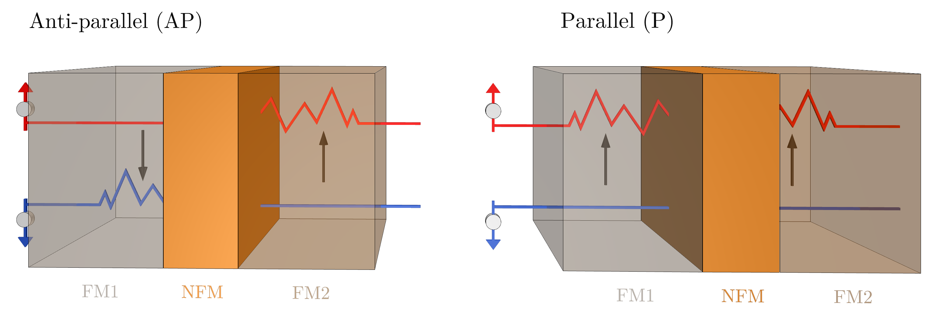
Figure 2.1: Illustration of spin-dependent electron scattering in a metallic multilayer structure demonstrating the GMR effect. Red arrows represent spin-up electrons, blue arrows denote spin-down electrons, and black arrows indicate the magnetization direction. In the AP configuration (left), both spin channels experience greater scattering, leading to higher resistance. In the P configuration (right), majority-spin electrons encounter less scattering, resulting in lower resistance.
2.2.2 Tunnel Magnetoresistance

TMR is a magnetoresistive phenomenon observed in MTJs, where a thin insulating barrier, most commonly crystalline MgO, separates two FMs electrodes. The junction resistance depends on the relative alignment of the magnetization in the ferromagnetic layers, analogous to the GMR effect. In the P configuration, spin-polarized electrons can tunnel more efficiently due to the matching density of states (DOS) at the Fermi level in both layers, resulting in higher conductance and lower resistance. In contrast, when the magnetization is AP, the spin states become misaligned, reducing the tunneling probability and thus increasing the resistance.

TMR can be understood as the counterpart of the GMR effect, observed when the metallic spacer layer in a spin valve is replaced with a thin insulating tunnel barrier, forming an MTJ. The phenomenon was initially discovered by Jullière in 1975 using Fe/GeOx/Co junctions, where a conductance change of approximately 14 % was observed at 4.2 K  [14]. Due to its limited magnitude, the effect initially attracted little attention. However, after the discovery of GMR, TMR was revisited, and significantly stronger effects (10–20 % at room-temperature) were soon reported using amorphous Al\(_2\)O\(_3\) barriers between Co or CoFe ferromagnetic layers  [48, 61]. For comparison, modern MTJs based on ferromagnets typically exhibit TMR ratios between 50–200 % at room-temperature, with record values exceeding 600 %  [53].

The key functional element of a MRAM cell based on the TMR effect is the MTJ. In such junctions, spin-dependent tunneling occurs because the probability of an electron tunneling through the barrier depends on the availability of the same spin states in the destination layer. Since electron spin is conserved mainly during tunneling, electrons can only tunnel into electronic states of the same spin orientation (see Figure 2.2). A transition from the P configuration (Figure 2.2 (left panel)) to the AP configuration (Figure 2.2 (right panel)) effectively inverts the spin bands in one electrode, leading to a mismatch in the spin-resolved DOS between the two layers. As a result, the overall tunneling current is reduced, leading to a measurable change in resistance.

The theoretical foundation of TMR was first described by Jullière  [14], who proposed a simple model based on two key assumptions:

  • (i) The electron spin is conserved in the tunneling process. This implies that the tunneling of spin-up and spin-down electrons is an independent process, and that the carriers tunnel from the first film are accepted by empty states of the same spin orientation in the second film.

  • (ii) The tunneling conductance \(G_\mathrm {P}\) and \(G_\mathrm {AP}\) are proportional to the product of the spin-resolved density of states of the two ferromagnetic layers.

Based on these assumptions, the conductance in the P and AP configurations are expressed as:

\begin{align} G_{\mathrm {P}} & \propto N_1^\uparrow N_2^\uparrow + N_1^\downarrow N_2^\downarrow = 1 - N_1^\uparrow -N_2^\uparrow + 2N_1^\uparrow N_1^\uparrow , \\ G_{\mathrm {AP}} & \propto N_1^\uparrow N_2^\downarrow + N_1^\downarrow N_2^\uparrow = N_1^\uparrow +N_2^\uparrow - 2N_1^\uparrow N_1^\uparrow , \end{align}

(image)

Figure 2.2: Illustration of spin-dependent tunneling responsible for the TMR effect. In the P configuration (left), spin-polarized electrons tunnel into available states of the same spin orientation in the second ferromagnetic layer, resulting in high conductance. In the AP configuration (right), spin mismatch reduces the tunneling probability, leading to low conductance.

where \(N^\uparrow \) and \(N^\downarrow = 1 - N^\uparrow \) are the spin-up and spin-down fractions of the density of states at the Fermi level, and subscripts 1 and 2 refer to the first and second ferromagnet, respectively.

Introducing the spin polarization of the conduction electrons as:

\begin{equation} P = \frac {N^\uparrow - N^\downarrow }{N^\uparrow + N^\downarrow } = 2N^\uparrow - 1, \end{equation}

we can write the TMR ratio as:

\begin{equation} \mathrm {TMR} = \frac {G_{\mathrm {P}} - G_{\mathrm {AP}}}{G_{\mathrm {AP}}} = \frac {R_{\mathrm {AP}} - R_{\mathrm {P}}}{R_{\mathrm {P}}} = \frac {2P_1 P_2}{1 - P_1 P_2}. \end{equation}

For symmetric junctions where \(P_1 = P_2 = P\), this simplifies to:

\begin{equation} \mathrm {TMR} = \frac {2P^2}{1 - P^2}. \end{equation}

While Jullière’s model provides intuitive insight into the spin-filtered nature of tunneling, it assumes incoherent tunneling and does not account for band symmetries. In practice, the tunneling process significantly depends on the symmetry of the electron wavefunctions. In MTJs with amorphous Al\(_2\)O\(_3\) barriers, tunneling is incoherent, and Jullière’s model is applicable. However, for crystalline barriers such as MgO, only electrons with specific Bloch state symmetries (e.g., \(\Delta _1\)) contribute to tunneling. This symmetry filtering effect strongly suppresses conductance in the AP state and leads to much higher TMR ratios  [62].

This behavior is reflected in the angular dependence of the conductance, modeled by Slonczewski  [63]:

\begin{equation} G(\theta ) = \frac {G_{\mathrm {P}} + G_{\mathrm {AP}}}{2} + \frac {G_{\mathrm {P}} - G_{\mathrm {AP}}}{2} \cos \theta = \frac {G_{\mathrm {P}} + G_{\mathrm {AP}}}{2} \left (1 + \frac {\mathrm {TMR}}{2 + \mathrm {TMR}} \cos \theta \right ), \label {eq::angular_conductance} \end{equation}

where \(\theta \) is the angle between the magnetizations in the two ferromagnetic layers. Maximum conductance is achieved at \(\theta = 0\) (P), and minimum at \(\theta = \pi \) (AP)  [36, 64, 65].

Although discovered before GMR, practical applications of TMR became viable only in the mid-1990s. In 1995, Moodera et al.  [48] and Miyazaki et al.  [66] independently demonstrated room-temperature TMR in junctions with amorphous Al\(_2\)O\(_3\) barriers, achieving TMR ratios of 20-30 %  [61]. This milestone catalyzed extensive research into MTJ-based memory devices. Further improvements in materials and deposition processes enabled TMR values of up to 70.4 % with Al\(_2\)O\(_3\) barriers  [67].

A major theoretical breakthrough came in 2001, when Butler et al.  [49] and Mathon et al.  [50] predicted that coherent tunneling through crystalline MgO barriers could yield TMR ratios exceeding 1000 %. These predictions were experimentally validated in 2004 by Parkin et al.  [25] and Yuasa et al.  [26], who reported room-temperature TMR values of 180–220 % in epitaxial Fe/MgO/Fe junctions. Subsequent work highlighted the critical role of Ar pressure during MgO sputtering, which affects barrier crystallinity and overall performance  [68]. Continued optimization of interface engineering and thermal annealing led to record-breaking TMR values of 410 %  [69] and 604 % at room-temperature (and up to 1144 % at 4.2 K) in CoFeB/MgO stacks  [53].

Today, MgO-based MTJ structures are central to commercial STT-MRAM technologies due to their high TMR, scalability, and CMOS compatibility.