« PreviousUpNext »Contents
Previous: 4.2 The non-radiative multiphonon (NMP) model Top: 4 Modeling of charge trapping phenomena Next: 5 Electrical characterization of interface defects in GaN-based MIS-HEMTs
4.3 Extraction of the activation energy and  from experimental data
In this section we introduce two data analysis methods that assume a constant  , dedicated to the extraction of single–valued and
distributed activation energies. We test the methods on three datasets, simulated using Eq. (4.3) and Eq. (4.6). We reproduce the
, dedicated to the extraction of single–valued and
distributed activation energies. We test the methods on three datasets, simulated using Eq. (4.3) and Eq. (4.6). We reproduce the  transients during stress in the case of a single–valued
  of 0.3 eV (labeled “single–state”), the case of two
trap states with energies 0.2 eV and 0.4 eV (“multi–state”), and a normal distribution of activation energies with mean
of 0.3 eV (labeled “single–state”), the case of two
trap states with energies 0.2 eV and 0.4 eV (“multi–state”), and a normal distribution of activation energies with mean  0.3 eV and standard deviation
  0.1 eV (“distributed”), from 10 µs to 100 s. We choose a
pre–factor = 50 ns and various temperatures between
−100 °C and 100 °C. The transients obtained in this way are shown in Fig. 4.4.
0.1 eV (“distributed”), from 10 µs to 100 s. We choose a
pre–factor = 50 ns and various temperatures between
−100 °C and 100 °C. The transients obtained in this way are shown in Fig. 4.4.
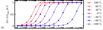
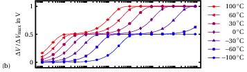

Figure 4.4: Simulated transients with  50 ns at temperatures from −100 °C
to 100 °C over seven decades. We assume a single–valued of 0.3 eV (a), two defect states with single–valued
of 0.2 eV and 0.4 eV (b), and a normal dis-
tribution of activation energies with mean 0.3 eV and standard deviation 0.1 eV (c).
50 ns at temperatures from −100 °C
to 100 °C over seven decades. We assume a single–valued of 0.3 eV (a), two defect states with single–valued
of 0.2 eV and 0.4 eV (b), and a normal dis-
tribution of activation energies with mean 0.3 eV and standard deviation 0.1 eV (c).
Furthermore, we discuss the effect of a non–constant on the data. The methods described here are applied
in Chapter 5 to our experimental data.
4.3.1 Extracting single–valued activation energies
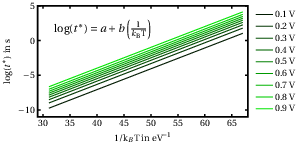
We present here a direct, simple way to evaluate the activation energy from a set of recovery transients at different temperatures, based on the Arrhenius equation. We choose few values of voltage shift,  , included in the range of our dataset. In our
example, we take nine values between 0 V and 1 V. For each recovery transient we extract the time
, included in the range of our dataset. In our
example, we take nine values between 0 V and 1 V. For each recovery transient we extract the time  at the extraction voltage . In this way we obtain a set of as a function of temperature and . For each extraction voltage we perform a
linear fit of log
at the extraction voltage . In this way we obtain a set of as a function of temperature and . For each extraction voltage we perform a
linear fit of log as a function of
  , the Arrhenius plot, which is shown in
Fig. 4.5. According to Eq. (4.3), the slope of the fitting line is the activation energy and the offset gives the pre–factor . Finally, an average over the results at various gives an estimate for and [54].
, the Arrhenius plot, which is shown in
Fig. 4.5. According to Eq. (4.3), the slope of the fitting line is the activation energy and the offset gives the pre–factor . Finally, an average over the results at various gives an estimate for and [54].


Next, we test the Arrhenius analysis of the simulated data. The results are shown in Fig. 4.6 for various values of . We note that this method provides an
accurate energy value for all values when the distribution is
single–valued. Also for two single–valued states (or multi–state), it is possible to distinguish two regions where the two distinct activation energies are correctly estimated. On the contrary, if is broadly distributed the results at various can be very different. In this case, the
smallest and largest give an error in the activation energy of
about 30%. Nevertheless, we note that the extracted activation energy as a function of is symmetric around its mean value, in our
example 0.3 eV. Therefore the average over all extraction voltages gives the correct mean activation energy  . Visually, we can determine the mean value as the symmetry axis in Fig. 4.6a. Unfortunately, this is rarely possible with real data. In the first place, noise might conceal this feature. Another reason is that the measurement window
should be large enough to reveal the whole shape like in Fig. 4.6a, which is impossible to know a priori. Therefore, this method might give just a rough
estimate of the real value. Regarding the pre–factor , the error in this case is larger than for the activation
energy. In fact, the fitted values have the correct order of magnitude but they can be 35% off the original .
. Visually, we can determine the mean value as the symmetry axis in Fig. 4.6a. Unfortunately, this is rarely possible with real data. In the first place, noise might conceal this feature. Another reason is that the measurement window
should be large enough to reveal the whole shape like in Fig. 4.6a, which is impossible to know a priori. Therefore, this method might give just a rough
estimate of the real value. Regarding the pre–factor , the error in this case is larger than for the activation
energy. In fact, the fitted values have the correct order of magnitude but they can be 35% off the original .

Figure 4.6: Activation energy (a) and pre–factor (b) extracted from the simulated data. The original
values are a single–valued  0.3 eV, a multi–state defect with
  0.2 eV and
  0.4 eV, and a normal distribution of ener-
gies with mean 0.3 eV and standard deviation 0.1 eV. We use a constant of 50 ns. The average over for and are shown in the legend.
0.4 eV, and a normal distribution of ener-
gies with mean 0.3 eV and standard deviation 0.1 eV. We use a constant of 50 ns. The average over for and are shown in the legend.
In conclusion, this method provides an estimate of the mean value of the activation energy, but it does not give any insight into the actual range of its distribution. Therefore, this analysis is sufficient if the activation energy has a precise, single value, but it
offers only partial information if is distributed across a broader range, which is the most
common situation for interface defects.
4.3.2 Extracting distributed activation energies
We present here a method to extract the distribution of activation energies associated with trapping events, which is based on the study of chemical reaction kinetics, proposed by Primak in 1955 [91]. In fact, the charge exchange event responsible for
the device drift causes the modification of certain chemical bonds at the AlGaN/SiN interface. We can therefore think of the capture process as a chemical reaction which transforms a reactant, the empty trap, into a product, the filled trap state. This approach can
be described mathematically with a differential equation. Indicating the reactant concentration as a quantity depending on the activation energy,  , its time evolution is given by the differential
equation
, its time evolution is given by the differential
equation

where we assume for simplicity first–order kinetics, with  as its temperature–activated rate constant,
obeying Eq. (4.3). The solution of the differential equation is
as its temperature–activated rate constant,
obeying Eq. (4.3). The solution of the differential equation is
![(4.11) \begin{equation} g (t, E_A) = g (t=0) \; \mr {exp}\left [-\frac {t}{\tau _0} \mr {exp}\left ( - \frac {E_A}{k_\mr {B}\mr {T}} \right )\right ]
\end{equation}](lateximages/lateximage-644.svg)
which can be written as

where the function  is called the characteristic isothermal
annealing function. It is a monotonically increasing function of the activation energy, with a rising transient around the characteristic activation energy
is called the characteristic isothermal
annealing function. It is a monotonically increasing function of the activation energy, with a rising transient around the characteristic activation energy

The width of the rising transient is directly proportional to [91]. Since is usually small, the characteristic isothermal
annealing function can be approximated with a step function in  with a small error [92].
Furthermore, if we integrate the reactant concentration over energy, we obtain the density of active
defects,  :
:

In addition,  is actually the spectral density of defects that
play a role in this reaction. We call the spectral density
is actually the spectral density of defects that
play a role in this reaction. We call the spectral density  , which is the distribution in energy of
. As a consequence, we can calculate from the experimentally observed using Eq. (1.1) and
, which is the distribution in energy of
. As a consequence, we can calculate from the experimentally observed using Eq. (1.1) and

where  is the inverse of the coefficient .
This method therefore extracts the activation energy spectrum of the defect concentration. However, because of the approximation of by a step function, the result will be a
smooth function of the activation energy. For this reason this technique is not sensitive to sharp features in the spectrum.
The pre–factor can be extracted by a fit to the data taken at different
temperatures. Since we have the same temporal window for all measurements, we can calculate the defect density within an energy range determined by temperature through Eq. (4.13). The higher the temperature, the larger the values which are experimentally accessible. The optimal
is the value which gives a smooth spectrum when
connecting the parts at different temperature. We use a numerical algorithm in order to optimize according to this approach.
We begin the evaluation of the Primak method using the simulated dataset. The results are shown in Fig. 4.7 for the three cases introduced in Fig. 4.4. The mean value of the activation energy is always extracted accurately: 0.3 eV for the single–state and distributed cases, and for the multi–state we can
see two distinct peaks at 0.2 eV and 0.4 eV. The optimized value for is compatible with the original 50 ns within
an error of 30%.
A limitation of this method is the apparent standard deviation, which is different from zero even for the dataset simulated with a single–valued trap states. In this case  is around 25 meV. This is
an artifact of the analysis caused by the assumption on the characteristic isothermal annealing function. We can consider to be the energy resolution of the
Primak method.
is around 25 meV. This is
an artifact of the analysis caused by the assumption on the characteristic isothermal annealing function. We can consider to be the energy resolution of the
Primak method.
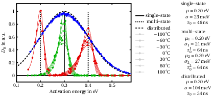
Figure 4.7: Activation energy distribution extracted from the simulated transients at various temperatures. The  values are scaled for better reading. The lines show
the original activation energy functions: the single–valued 0.3 eV (solid), the two single–valued 0.2 eV and 0.4 eV (dotted) and the normal distribution with mean 0.3 eV and standard deviation 0.1 eV (dashed).
values are scaled for better reading. The lines show
the original activation energy functions: the single–valued 0.3 eV (solid), the two single–valued 0.2 eV and 0.4 eV (dotted) and the normal distribution with mean 0.3 eV and standard deviation 0.1 eV (dashed).
4.3.3 Effects of a non–constant
As we discussed in Section 4.2.3, a broad distribution of trap types and the failure of the classical limit are two factors that can determine a non–constant over a set of data taken at different temperatures.
Having a more detailed look at the reaction kinetics, we find that in both cases the differential equation Eq. (4.10) is
no longer sufficient anymore to describe our system. Such equation means that the empty traps, with concentration  , are trapping electrons with a rate
  . Thus, they become filled traps, which have a concentration
  .
.
However, if at a certain temperature an additional defect “family”,  , becomes active, we do not have only the reaction from
to , but also that of to
, becomes active, we do not have only the reaction from
to , but also that of to  with a different rate constant
  . The two phenomena may even be competitive, because the electrons can be trapped in either
one or the other trap type. If the reaction is not limited by electron supply or other external factors, the observed time constant for electron capture is the average value between
. The two phenomena may even be competitive, because the electrons can be trapped in either
one or the other trap type. If the reaction is not limited by electron supply or other external factors, the observed time constant for electron capture is the average value between  and
and  . For example, if the defect type becomes active at high temperature, its time constant would
be probably longer than that for . In this way, we would obtain an increase of the effective
as a function of temperature.
. For example, if the defect type becomes active at high temperature, its time constant would
be probably longer than that for . In this way, we would obtain an increase of the effective
as a function of temperature.
On the other hand, if the reaction does not only happen through the classical intersection point (giving rise to the rate constant ), but also with tunnelling, we have an alternative way for the same reaction, with a different rate
constant  . In this case, the energetic barrier height is lower than the classical one, and this effect is stronger
the lower the temperature (see Fig. 4.3). As a consequence, the analysis of the data using Eq. (4.3) as explained in Section 4.3.1 would result in a temperature dependent activation energy, which means a temperature dependent slope in the Arrhenius plot.
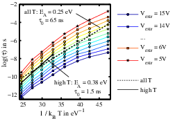
This might be a possible explanation for Fig. 4.8, which has been calculated for the MIS–HEMTs with fluorinated interface. The convex curvature of the
lines at low temperature indicates that there is a deviation from the classical Arrhenius interpretation [93]. We extract as the slope of a linear fit, by using the whole curve or just
the four highest values of temperature. As we would expect from Fig. 4.3b, the activation energy at high temperature is larger. Although many other explanations are possible,
charge exchange through tunnelling could be the reason of the non–linearity of the Arrhenius plot of these structures.
. In this case, the energetic barrier height is lower than the classical one, and this effect is stronger
the lower the temperature (see Fig. 4.3). As a consequence, the analysis of the data using Eq. (4.3) as explained in Section 4.3.1 would result in a temperature dependent activation energy, which means a temperature dependent slope in the Arrhenius plot.
This might be a possible explanation for Fig. 4.8, which has been calculated for the MIS–HEMTs with fluorinated interface. The convex curvature of the
lines at low temperature indicates that there is a deviation from the classical Arrhenius interpretation [93]. We extract as the slope of a linear fit, by using the whole curve or just
the four highest values of temperature. As we would expect from Fig. 4.3b, the activation energy at high temperature is larger. Although many other explanations are possible,
charge exchange through tunnelling could be the reason of the non–linearity of the Arrhenius plot of these structures.
We can add a third phenomenon that would result in a non–constant . At a certain temperature it might become possible
that the population transforms into a third state,  , having another, different rate constant
  and a higher activation energy than that of the main reaction. Let’s assume that the reaction
from to is not possible, or that it has an extremely large barrier. If we
can measure only the change from to but we are insensitive to , then we would observe less reactions than we would
expect, as some reactant are “blocked” in the third state. As a consequence, since the amount of to events depends on temperature, also the observed reaction
becomes temperature dependent, which will result in the observed curvature of the Arrhenius plot. This is often observed in biology studies, when a certain biological system (e.g., a protein) reacts with the system and transforms into something else; however, at
high temperature it can undergo a denaturation process which blocks the reaction. In this case, the Arrhenius plot log
and a higher activation energy than that of the main reaction. Let’s assume that the reaction
from to is not possible, or that it has an extremely large barrier. If we
can measure only the change from to but we are insensitive to , then we would observe less reactions than we would
expect, as some reactant are “blocked” in the third state. As a consequence, since the amount of to events depends on temperature, also the observed reaction
becomes temperature dependent, which will result in the observed curvature of the Arrhenius plot. This is often observed in biology studies, when a certain biological system (e.g., a protein) reacts with the system and transforms into something else; however, at
high temperature it can undergo a denaturation process which blocks the reaction. In this case, the Arrhenius plot log as a function of usually has a convex
shape [94].
as a function of usually has a convex
shape [94].
In conclusion, a non–constant could be due to different reasons [95]. More detailed
experiments are necessary in order to identify the true origin. The effect on the experimental data is clearly visible as the non–linearity of the Arrhenius plot. It should also be observed when we try to connect the data at different temperature with the Primak
method: if is temperature dependent, then we would not find a
single value which gives a smooth spectrum. However, this effect can be small because of the noise caused by the derivation of the data.
« PreviousUpNext »Contents
Previous: 4.2 The non-radiative multiphonon (NMP) model Top: 4 Modeling of charge trapping phenomena Next: 5 Electrical characterization of interface defects in GaN-based MIS-HEMTs