Impact of Charge Transitions at Atomic Defect Sites on Electronic Device Performance

3.2 Molecular dynamics

Molecular dynamics (MD) is a computational method, developed to simulate the motion of interacting particles over time in the framework of Newton’s equations of motion. For certain tasks, such as modeling the dynamics of atoms over a long time scale or for large system sizes, the description of interatomic forces with DFT can become impractically expensive, especially when employed in conjunction with hybrid functionals. In particular when quantum-mechanical interactions are negligible, more simplistic approaches such as classical MD might be sufficient. Classical MD is, for example, commonly used to simulate biological processes or calculate macroscopic thermodynamic properties of materials. The foundations of MD will be described in the following.

3.2.1 Newton’s equation of motion

The dynamics of particles are governed by the fundamental Newtonian equations of motion,

$$\begin{array}{}\text{(3.16)}& -{\mathrm{\nabla }}_{{\mathit{x}}_k}V(\mathit{x})={\mathit{F}}_k(\mathit{x})=m_k\frac{{\mathrm{d}}^2{\mathit{x}}_k(t)}{\mathrm{d}{t}^2},\end{array}$$

where $V(\mathit{x})$ is the potential energy as a function of the position of all particles, ${\mathit{F}}_k$ is the force on particle $k$, given as the gradient of the potential energy with respect to the coordinates of the $k^{\mathrm{th}}$ particle, $m_k$ is its mass, $\mathit{x}(t)=({\mathit{x}}_1(t),...,{\mathit{x}}_M(t))$ is the ensemble of positions of all $M$ particles and ${\mathit{x}}_k(t)$ the position of particle $k$ at time $t$.

The dynamics of an atomic system during an MD simulation are analyzed by solving Eq. (3.16) numerically. A commonly used method for this is the velocity Verlet algorithm [190, 191]. In this approach, the positions $\mathit{x}(t)$ and velocities $\mathit{v}(t)=\frac{d\mathit{x}(t)}{dt}$ after a time step $\mathrm{\Delta }t$ are evaluated by numerical integration of Eq. (3.16) based on a Taylor expansion. The equations for the positions and velocities of the particles in the system are given by

$$\begin{array}{}\text{(3.17)}& {\mathit{v}}_k(t+\mathrm{\Delta }t)={\mathit{v}}_k(t)+\frac{1}{2}({\mathit{a}}_k(t)+{\mathit{a}}_k(t+\mathrm{\Delta }t))\mathrm{\Delta }t\end{array}$$

$$\begin{array}{}\text{(3.18)}& {\mathit{x}}_k(t+\mathrm{\Delta }t)={\mathit{x}}_k(t)+{\mathit{v}}_k(t)\mathrm{\Delta }t+\frac{1}{2}{\mathit{a}}_k(t)\mathrm{\Delta }{t}^2,\end{array}$$

with the acceleration ${\mathit{a}}_k=\frac{d{\mathit{v}}_k(t)}{dt}$.

Within an iterative treatment, first, the initial velocities and positions of the particles in the system at $t=0$ have to be defined. After each time step, $\mathit{a}(t)$ is derived from Eq. (3.16) with a predefined interatomic potential (IP) $V(\mathit{x})$ that models the interactions between the atoms in the system. Following Eq. (3.17) and Eq. (3.18), ${\mathit{v}}_k(t+\mathrm{\Delta }t)$ and ${\mathit{x}}_k(t+\mathrm{\Delta }t)$ are updated after every successive time step. All MD simulations in this thesis were performed using the LAMMPS code [192]. This software package includes various algorithms to control the thermodynamic properties of the system.

3.2.2 Controlling the temperature

During the MD simulations, various thermodynamic properties of the atomic system can be kept constant to simulate realistic experimental conditions. The respective constraint properties define which statistical ensemble is sampled during the MD run [193]. For instance, canonical ensembles ($NVT$ ensembles) keep the number of particles $N$, the volume $V$ and the temperature $T$ in the system constant by exchanging energy with an external heat bath. In contrast, $NPT$ (isothermal-isobaric) ensembles keep the pressure $P$ instead of $V$ constant, while grand canonical ($\mu VT$) ensembles allow for the exchange of particles, while keeping the chemical potential $\mu$ constant.

In this thesis, MD calculations are used to generate amorphous structures by simulating a melt-and-quench procedure [156, 53, 54, 55, 194]. During this process, the system is first heated above its melting point, where it is equilibrated until the positions of the atoms fully randomize in the liquid phase. Subsequently, the melt is slowly cooled down to room temperature where it transitions into an amorphous solid. The temperature of the $NVT$ ensemble can be regulated by coupling the simulation cell to a thermostat, which corresponds to an algorithm that either removes or adds energy in a controlled way. This is achieved by either directly adjusting the velocities and consequently the kinetic energy of the atoms, or by modifying the governing Newtonian equations of motion, with the goal to keep the temperature of the system constant. For $NPT$ ensembles, additionally a barostat can be used to maintain constant pressure.

Several approaches for thermostat algorithms have been proposed. The simplest method rescales the velocity of the particles according to the desired kinetic energy. The Berendsen thermostat couples the system to a thermal bath, which allows for temperature fluctuations [195]. The Bussi-Donadio-Parrinello thermostat stochastically rescales the velocity by enforcing a kinetic energy which follows a Maxwell-Boltzmann distribution at canonical equilibrium [193]. The thermostat used for the melt-and-quench MD simulations in this thesis is the Langevin thermostat, which is based on the fundamental Langevin equation of motion. This equation was originally formulated in 1908 by Paul Langevin to model the random motion of particles in a fluid or a gas [196], but can as well be used to model $NVT$ ensembles during MD simulations [197]. The Langevin equation extends the basic MD formulation by two additional terms: a friction term for the treatment of viscous resistance and a stochastic term to model collisions with other particles in the system. The Langevin equation is given by [193]

$$\begin{array}{}\text{(3.19)}& m_k\frac{d^2{\mathit{x}}_k}{d{t}^2}=-{\mathrm{\nabla }}_{{\mathit{x}}_k}V(\mathit{x})-{\gamma }_k{m}_k\frac{d{\mathit{x}}_k}{dt}+{\eta }_k{\mathit{\xi }}_k,\end{array}$$

where ${\gamma }_i$ is the friction coefficient and ${\eta }_k$ determines the magnitude of the stochastic force ${\mathit{\xi }}_k$. The stochastic term is independent of the particle velocities and its three components along the Cartesian axis are uncorrelated. It is zero when averaged over time and changes the particles momentum within a Gaussian distribution with standard deviation ${\eta }_i$. The coefficients ${\eta }_k$ and ${\gamma }_k$ are correlated according to the fluctuation-dissipation theorem ${\eta }_k^2=2{\gamma }_k{m}_k{k}_{\mathrm{B}}T$.

During a quenching process of the melt-and-quench simulation to create amorphous structures, the desired temperature at each time step is linearly interpolated between the initial and final temperature. Although additionally applying a barostat would improve the description of realistic volume-temperature trends in the liquid phase, this would also significantly increase the computational costs [198]. Instead, to obtain realistic amorphous structures, the initial mass densities before the simulations were adapted to agree with experimental densities of amorphous thin films and the remaining stress of the quenched structures was released with DFT cell optimizations after the MD simulations. This procedure was used in this thesis to create amorphous silicon nitride ($a$-Si${}_3$N${}_4$:H) samples as discussed in Section 5.2.

3.2.3 Interatomic potentials

The remaining term in Eq. (3.16) and Eq. (3.19), $V(\mathit{x})$, which has not been discussed yet defines the physical interactions and dynamics of the system during the simulation. For this reason, choosing an appropriate $V(\mathit{x}(t))$ is crucial for a physically accurate description of the interactions and motions of the investigated particles. While it is possible to describe the forces of MD with DFT (ab initio MD), such calculations are computationally expensive and thus often not feasible for large system sizes or statistical analyses. In this thesis, MD is used to generate various initial amorphous structures for subsequent DFT calculations, where the precise interactions during high-temperature MD runs do not have to be analyzed in detail. Therefore, more approximate treatments, such as classical and machine-learned IPs, were considered sufficiently accurate for realistic structure creation. Both approaches for IPs will be briefly described in the following sections.

Classical interatomic potential

Classical IPs use non-quantum mechanical descriptions to model the interactions between atoms. These potentials are often referred to as empirical potentials, because they do not capture quantum mechanical interactions, but are parametrized to describe and predict chemical reactions or physical properties based on experiments and higher-level calculations. Classical IPs often include various terms to model different physical phenomena. Their simplified description of atomic interactions makes them computationally efficient and suitable for the simulation of large system sizes.

The classical IP that was used for several MD calculations in this thesis is ReaxFF [199]. This IP divides the system’s energy into various two-body and many-body contributions, including terms related to the bond order, over- and undercoordination, valence angle, torsion angle, conjugation effects, nonbonded van der Waals interactions and Coulomb interactions.

$$\begin{array}{}\text{(3.20)}& \begin{array}{rl}{E}_{\mathrm{system}}=E_{\mathrm{bond}}& +E_{\mathrm{over}}+E_{\mathrm{under}}+E_{\mathrm{val}}+E_{\mathrm{pen}}+\\ & +E_{\mathrm{tors}}+E_{\mathrm{conj}}+E_{\mathrm{vdWaals}}+E_{\mathrm{Coulomb}}\end{array}\end{array}$$

Since the first ReaxFF IP was developed, multiple ReaxFF force fields have been published for different atomic compositions. This is necessary because the parametrization of the respective terms has to be done individually for each atomic system being investigated. A major strength of ReaxFF is its ability to model both bond formation and breaking during the MD run, which is crucial for generating realistic amorphous structures with MD using the melt-and-quench technique [15, 4].

Machine-learning interatomic potential (MLIP)

An alternative approach for defining an IP that aims to combine the efficiency of classical MD with the accuracy of DFT is the MLIP. In this method, an ML algorithm is used to train an IP based on accurately calculated properties from various atomic configurations. These properties includes energies, forces and stress tensors, which are typically obtained at the DFT level. Several approaches have been proposed for the underlying ML model. In this thesis, the Gaussian approximation potential (GAP) [200] method is used to generate the MLIP. Alternative options to train MLIPs include artificial neural networks [201], message-passing network [202] and moment tensor potentials [203].

The GAP potential learns the PES (see Section 2.1.2) of a system as a function of the atomic positions. Thereby, different mathematical representations of atomic environments, known as descriptors, are used to link the training dataset composed of various atomic structures with the ML model. Descriptors relate the positions of atoms to energies on the PES and must be invariant under rotation and translation of the entire atomic configuration and permutations of atoms of the same type. Local descriptors depend on the neighboring atomic environment within a cutoff radius. GAP employs a set of local descriptors for the training of the PES, neglecting long-range interactions beyond the cutoff. In addition to simple geometrical 2-body and 3-body descriptors, such as bond lengths or angles, GAP also uses the more sophisticated smooth overlap of atomic positions (SOAP) descriptor [204]. SOAP captures the local environment around a single atom by considering the positions of neighboring atoms and approximates the atomic neighbor density with Gaussian functions. It is designed to provide a smooth and differentiable description of the PES.

The total energy, $E_{\mathrm{total}}$, of the system as described by the GAP is given by the sum of the individual energy contributions $ϵ({\mathit{q}}_{k_d}^{(d)})$ from the local environments ${\mathit{q}}_{k_d}^{(d)}$ represented by the descriptor of type $d$ [200, 205]

$$\begin{array}{}\text{(3.21)}& E_{\mathrm{total}}=\sum _{k_d,d}({\delta }^{(d)}{)}^2{ϵ}^{(d)}({\mathit{q}}_{k_d}^{(d)}).\end{array}$$

Here, $k_d$ ranges over all ensembles analyzed by the respective descriptor $d$, e.g. over all atom pairs (triplets) for two-body (three-body) descriptors. ${\delta }^{(d)}$ is a scaling parameter that depends on the type of the respective descriptor, with two-body descriptors typically having the largest $\delta$ as they contribute most to the total energy. For each descriptor, the local energy contribution is determined by a linear combination of specific kernel functions $K$

$$\begin{array}{}\text{(3.22)}& {ϵ}^{(d)}({\mathit{q}}^{(d)})=\sum _{t=1}^{N_t^{(d)}}{\alpha }_t^{(d)}{K}^{(d)}({\mathit{q}}^{(d)},{\mathit{q}}_t^{(d)}).\end{array}$$

$K$ quantifies the similarity between input configuration $\mathit{q}$ and the $t^{\mathrm{th}}$ training configuration ${\mathit{q}}_t$ as schematically depicted in Fig. 3.1.

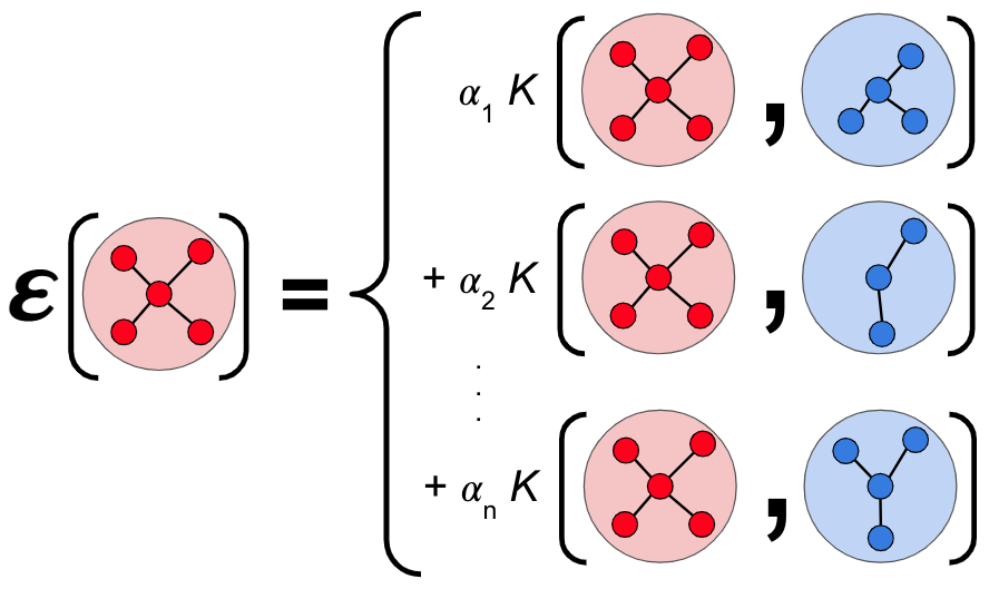
The kernel compares the input structure $\mathit{q}$ with a training configuration ${\mathit{q}}_t$ and gives a value proportional to the similarity. ${\alpha }_t^{(d)}$ are weighting coefficients, optimized during the training process of the GAP to minimize the error between the potential energies of the reference data and the potential energy as predicted by the GAP.

Training of an MLIP

In addition to the total energies and atomic positions of the structures, the atomic forces and stress tensors, which are derivatives of the total energy with respect to the atomic positions and the lattice deformation [206], can also be incorporated into the GAP training process. Including the stress tensor in the training set is important to make the MLIP applicable to structures with different mass densities. The ability of the MLIP to predict properties from DFT improves systematically with the size of the training dataset $N_t$ [200, 194, 207]. To improve the accuracy of the GAP, it is also beneficial to include calculations of different structure types in the training dataset. This may involve amorphous and crystalline systems with different densities, as well as dimers of all permutations of atomic compositions with varying interatomic distances.

The training process of the MLIP is done in an iterative manner as schematically shown for amorphous structure creation in Fig. 3.2 [194].

Initial amorphous structures are generated by simulating a melt-and-quench procedure with a classical force field and their forces, energies and stress tensors are subsequently recalculated with DFT. The resulting properties, along with the according atomic positions of the respective structures, serve as the training dataset for the first generation of the GAP. During the training process, the fitting coefficients of Eq. (3.22) are optimized to minimize the energy difference of the GAP with the input data. Subsequently, MD simulations are performed with this GAP to create new amorphous structures. The forces, energies and stress tensors of these structures are again recalculated with DFT and added to the training dataset. These steps are iteratively repeated until sufficient agreement with DFT results and experimental data is achieved. MLIPs can also be trained for dynamic processes such as the thermal oxidation of Si [207].

When early generations of the GAP are employed for MD melt-and-quench simulations, the generated structures may exhibit unphysical behavior such as clusters and chains of atoms or structural inhomogeneities. After each training iteration, the GAP learns more about the atomic interactions due to the enlarged training dataset, improving its physical description to approach the one of DFT. The similarity between the final GAP and DFT is shown in a correlation plot in Fig. 3.3, where the energies (a) and forces (b) of 1000 different liquid and amorphous Si${}_3$N${}_4$ structures from GAP and DFT calculations are compared [194]. More details about the GAP training parameters and the training dataset can be found in [194]. Hereby, every point in the plot represents a different amorphous (green) or liquid (blue) structure.

The sample structures in this analysis were not part of the training data of the GAP and were randomly selected from an MD run. The mean absolute errors (MAE) are 8 meV/atom for the total energies and 0.26 eV/Å  for the forces, respectively, which is in the range of other GAP MLIPs in literature. While these errors might seem significant, the goal of the GAP is not to compare the absolute values of total energies with DFT, since these are arbitrary. More importantly, because the GAP description of forces and energies correlates linearly with DFT and shows no systematic error, it is a qualitatively accurate representation of full quantum-mechanical calculations of structural properties.