« PreviousUpNext »Contents
Previous: 3.2 Electromigration in Bulk Metals Top: 3 Models Next: 3.4 Continuum Mechanical Model
3.3 Electromigration at Interfaces
Interfaces regarding EM are the domains which connect either bulk metal domains of the same metal kind or bulk materials of two different kinds. In the second case the interface can separate two conducting materials or a
conducting material from a nonconducting material. In all three cases the interface can have a diffusion coefficient higher then the coefficient of the bulk material or a lower equilibrium concentration.
How to handle this behavior is shown in the two next subsections. This is followed by a subsection explaining the case of an interface between two conducting materials, where the interface can have a segregation behavior.
3.3.1 Fast Diffusivity Paths at Interfaces
The crystal structure is highly disturbed at interfaces as there crystals with different orientations or even crystals with other lattice kinds or lattice parameters meet. This leads to atoms with a decreased binding energy compared
to the atoms located in the undisturbed lattice of a bulk material. This increases the probability for those atoms to jump and therefore increases also the diffusion coefficient as shown by Sørensen et al. [133].
This jumping is limited by the two-dimensional plane of the interface embedded in the 3D space. Therefore, interfaces show a highly direction depending diffusion coefficient giving it the form of a second order tensor. Since for
interfaces the real thickness can hardly be defined, for simulation normally the interface is modeled by a domain with a small but finite thickness. As a smaller thickness leads to a higher amount of mesh elements to ensure a
reasonable mesh quality, a thicker layer is desired. For these reasons in the further description of the modeling of fast diffusivity paths a thickness  is chosen to be the modeled interface thickness and its influence is pointed
out.
is chosen to be the modeled interface thickness and its influence is pointed
out.
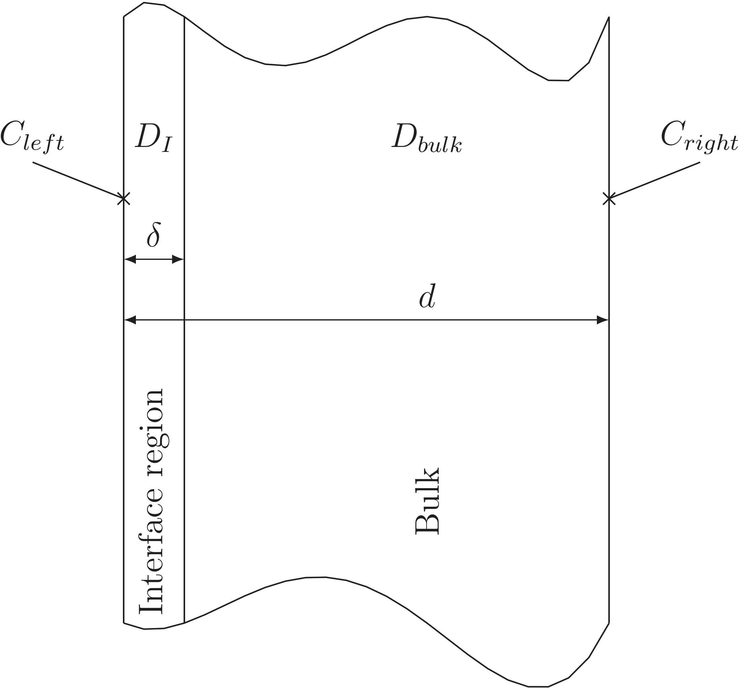
Figure 3.1.: Segment with an interface domain and a neighboring bulk domain for the diffusion coefficient calculation.
In Section 2.1.3 the effective diffusion coefficient was calculated by (2.9), where the diffusion in the bulk was taken to be negligibly small compared to the diffusion in the  . Extending this equation for a finite diffusion coefficient in the
bulk leads to the expression for the effective diffusion coefficient [136] for a structure shown in Figure 3.1 with an interface and an bulk segment.
. Extending this equation for a finite diffusion coefficient in the
bulk leads to the expression for the effective diffusion coefficient [136] for a structure shown in Figure 3.1 with an interface and an bulk segment.

If the effective diffusion coefficient is known from experimental data this equation can be rearranged to

giving a functional dependence on the interface thickness and the interface diffusion coefficient.
This value is the diffusion coefficient in the directions parallel to the interface surface, whereas the value perpendicular to the interface surface is given by the bulk diffusion coefficient, leading to a tensor form of the diffusion
coefficient. For very small interface thicknesses this distinction of the direction is not needed, shown by the following gedankenexperiment. The flow of vacancies perpendicular to the interface is calculated for the structure shown in
Figure 3.1 for predetermined vacancy concentrations at the left and right side of the structure in the following way:

left

right
For the case of an infinite small interface  this leads to

whereas for a finite interface it results in

Setting both equations to the concentration difference assumed at the beginning, substituting  form (3.18) and calculating the
relative error gives
form (3.18) and calculating the
relative error gives

and establishes a rule under which the directional dependence of the diffusion can be neglected.
3.3.2 Interfaces with Lower Equilibrium Concentrations
Interfaces can have, due to their disorder, a lower vacancy equilibrium concentration, as in the bulk, where vacancies can be easily filled by surrounding atoms as their binding energy is lower there. This is modeled by an extra region with a lower equilibrium concentration between the bulk materials in the Rosenberg-Ohring term inside the domain in contrast to the surrounding domains. This phenomenon is particularly important at interfaces between voids and bulk materials, as there at one side a lattice is formed, whereas on the other side no material is present. Therefore, this behavior is given special attention in the phase field model for voids in Section 3.6.
3.3.3 Segregation Model
Surfaces between different conducting materials play a special role in EM. The current at these interfaces passes from one conducting material to another. But for vacancies passing the interface can be hindered leading to a
segregation in the vicinity of those interfaces. The segregation at interfaces was modeled by Lau et al. [90] based on the work of Grove et al. [52]. The interface in this model makes use of a trap density  where the filled traps are denoted by
  and the empty ones by
  . These traps are dynamically coupled to the bulk
materials’ concentrations
. These traps are dynamically coupled to the bulk
materials’ concentrations  and
and  by the flows

and

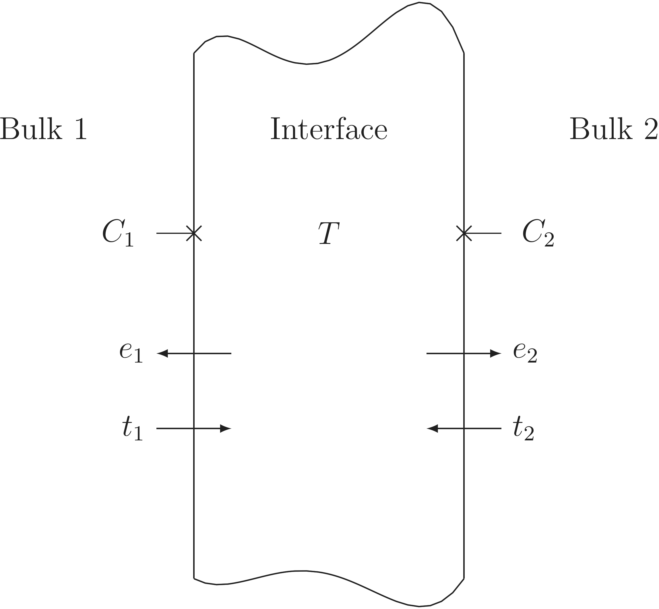
Figure 3.2.: Schematics for the derivation of the segregation model according to [90].
respectively, where the  are the emission probabilities and
  are the trapping probabilities. These equations
can be put together to calculate the time derivative of the filled trap density by
are the trapping probabilities. These equations
can be put together to calculate the time derivative of the filled trap density by

With the assumption of an equilibrium, where the filled trap density is constant in time, (3.26) can be rearranged to

Using the fact that the filled and the empty traps are the sum of the total traps density

leads to the filled trap density

where  and
and  are given by


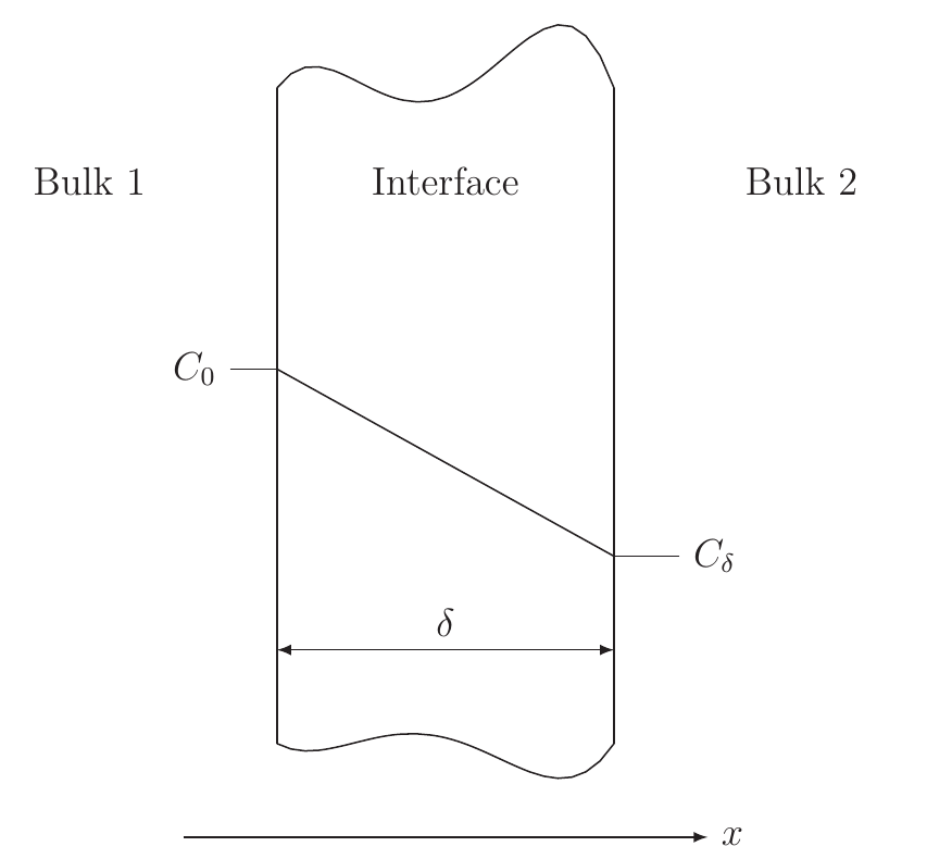
Figure 3.3.: Schematics for the derivation of the segregation model as an infinite thin representation of an interface with thickness.
Inserting the filled trap density in the flow equations (3.24) and (3.25) keeping in mind (3.28) results in

with  named the transport coefficient, and
  the segregation coefficient. In the calculations the segregation coefficient is taken to be
constant.
the segregation coefficient. In the calculations the segregation coefficient is taken to be
constant.
In the following it is shown that the segregation model can also be used for an infinitely thin representation of a domain with a thickness and a diffusion coefficient , if is set to one. As the domain thickness is small compared to a characteristic length (e.g.
grain radius) the concentration profile in this thin domain can be approximated with the first order Taylor expansion ( . Figure 3.3)

where  can be identified as the concentration in the left
bulk material equaling and
can be identified as the concentration in the left
bulk material equaling and  as the concentration in the right bulk
material . Differentiation of (3.33) with respect to
as the concentration in the right bulk
material . Differentiation of (3.33) with respect to  and putting the result in the flux driven by diffusion (cf. (3.11)) regarding only the
direction leads to
and putting the result in the flux driven by diffusion (cf. (3.11)) regarding only the
direction leads to

giving exactly the result of the segregation model shown above. It should be emphasized that this interface has in the limit of an infinitely small thickness no capability to store any vacancies, as all the flow from the left side is compensated by an equal flow on the right side. This behavior has to be taken into account as for mechanical stress calculations in FEM there is no easy way to handle a volume decrease due to the pile-up of vacancies in infinitely thin interfaces exhibiting zero volume.
« PreviousUpNext »ContentsPrevious: 3.2 Electromigration in Bulk Metals Top: 3 Models Next: 3.4 Continuum Mechanical Model