« Previous Up Next »Contents
Previous: 3.5 Void Nucleation Top: 3 Models Next: 4 Numerical Implementation

3.6 Void Evolution

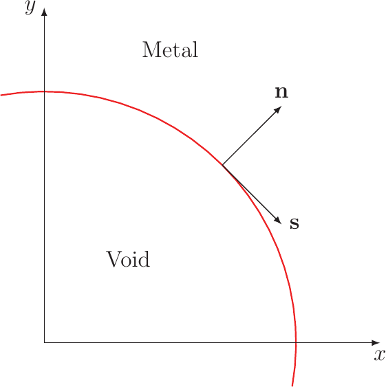
The void evolution phenomenon causes degradation by increasing the resistance of an interconnect after the void has nucleated. This process is modeled by equations tracking the movement of an interface, representing the boundary between the interconnect metal and the void [73]. For the calculations Bhate et al. [8, 9] introduced a local coordinate system at the void surface (shown in Figure 3.4). The chemical potential of the surface, when no current is present, is given by [58]:

$(3.47) \{begin}{gather} \mu _{\mathrm {s}}=\Omega (-\gamma _{\mathrm {s}}\kappa +W) \mathref {(3.47)} \{end}{gather}$

$\kappa$ is the surface curvature, $\gamma _{\mathrm {s}}$ is the surface energy, and $W$ is the elastic strain energy density.

$(3.48) \{begin}{gather} W=\displaystyle \frac {1}{2}\pmb {\epsilon }:\pmb {\sigma }=\frac {1}{2}\pmb {\epsilon }:\mathrm {\b {C}}\pmb {\epsilon } \mathref {(3.48)} \{end}{gather}$

The “double-dot” operator is defined for the tensors $\b {A}$ and $\mathrm {\b {B}}$ by

$(3.49) \{begin}{gather} \displaystyle \mathbf {A}:\mathbf {B}=\sum _{i,j}A_{ij}B_{ij} \mathref {(3.49)} \{end}{gather}$

and $A_{ij}, B_{ij}$ stands for the components of the tensor $\b {A}$ and $\mathbf {B}$ , respectively. The flux parallel to the surface is driven by the chemical potential of the surface and the EM flux summing up to

$(3.50) \{begin}{gather} J_{\mathrm {s}}=-\displaystyle \frac {D_{\mathrm {s}}\delta _{\mathrm {s}}}{k_{\mathrm {B}}T}\ \Bigl (\frac {\partial \mu _{\mathrm {s}}}{\partial s}-eZ^{*}\frac {\partial \phi _{\mathrm {E}}}{\partial s}\Bigr ), \mathref {(3.50)} \{end}{gather}$

where the derivatives are taken along the interface and the surface diffuse coefficient $D_{\mathrm {s}}$ obeys an Arrhenius law

$(3.51) \{begin}{gather} D_{\mathrm {s}}=D_{\mathrm {s},0}\displaystyle \exp \Bigl (-\frac {E_{\mathrm {A}}}{k_{\mathrm {B}}T}\Bigr ) . \mathref {(3.51)} \{end}{gather}$

Furthermore, a flux normal to the surface due to a flow of vacancies from the bulk to the surface, reasoned by the difference of the chemical potentials in the bulk and at the surface, is given by

$(3.52) \{begin}{gather} J_{\mathrm {n}\mathrm {v}}=\hat {D}(\mu _{\mathrm {b}\mathrm {v}}-\mu _{\mathrm {s}\mathrm {v}}), \mathref {(3.52)} \{end}{gather}$

where $\hat {D}$ controls the rate of vacancy exchange between the bulk and the surface. For the chemical potential of the vacancies at the surface the negative chemical potential of the surface is taken as given by (3.47). For the bulk the chemical potential is given by:

$(3.53) \{begin}{gather} \mu _{\mathrm {b}\mathrm {v}}=k_{\mathrm {B}}T \ln \Bigl (\displaystyle \frac {C_{\mathrm {v}}}{C_{\mathrm {v},\mathrm {e}\mathrm {q}}}\Bigr ) -(f-1)\Omega \sigma \mathref {(3.53)} \{end}{gather}$

Given these equations and considering the mass conservation the normal velocity of the void surface can be expressed as:

$(3.54) \{begin}{gather} v_{\mathrm {n}}=-\displaystyle \frac {\partial J_{\mathrm {s}}}{\partial s}-J_{\mathrm {n}\mathrm {v}} \mathref {(3.54)} \{end}{gather}$

A problem with this model arises from the need to track the interface for every simulation time step, if the FEM is employed as the simulation domains have to be separated in a void region and a metal region and these regions change in shape. The metal region has to be remeshed for every time step, increasing the simulation complexity. Therefore a model was proposed by Bhate et al. [9] according to Cahn et al. [19], where the boundary between the void and the metal is not modeled by a sharp interface, but by a thin region called the diffuse interface. To distinguish between the three regions a function called the order parameter $\phi (\vec {x},\ t)$ is defined, which has the property to be 1 in the metal decreasing smoothly in the interface region and being $-1$ in the void region. The free energy functional is defined by

$(3.55–3.56) \{begin}{gather} \displaystyle \mathcal {F}(\phi ,\ \pmb {\epsilon })=\int F(\phi ,\ \nabla \phi ,\ \pmb {\epsilon })\mathrm {d}V. \mathref {(3.55)} \\ =\displaystyle \int \ \Bigl (\frac {2\gamma _{\mathrm {s}}}{\epsilon _{\mathrm {p}\mathrm {f}}\pi }\ \Bigl (f(\phi )+\frac {1}{2}\epsilon _{\mathrm {p}\mathrm {f}}^{2}|\nabla \phi |^{2}\Bigr )\ +W(\pmb {\epsilon },\ \phi )\Bigr )\mathrm {d}V. \mathref {(3.56)} \{end}{gather}$

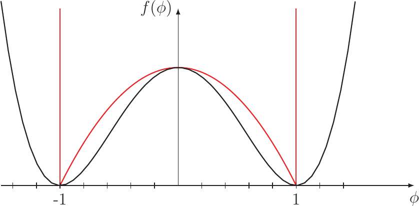
Figure 3.5.: Two shapes proposed for the bulk free energy function $f(\phi )$ . The quadratic double well potential in black and the double obstacle potential in red.

where $W(\pmb {\epsilon },\ \phi )$ is the elastic strain energy density given by

$(3.57) \{begin}{gather} W(\displaystyle \pmb {\epsilon },\ \phi )=\frac {1}{2}\pmb \epsilon :\mathrm {C}(\phi )\pmb \epsilon \mathref {(3.57)} \{end}{gather}$

and $f(\phi )$ is the bulk free energy function. The shape of this function has to meet the requirements to be positive everywhere and zero for $\phi$ equaling one or minus one. Two shapes proposed by different authors are shown in Figure 3.5. The black line is the quadratic double well potential proposed by Mahadevan et al. [99]. The red line is the double obstacle potential proposed by Oono et al. [106]. This potential was employed by Bhate et al. [9] in a calculation utilizing the finite-difference method, as it reduces the computational effort only to those areas, where the interface is located and the potential has a finite value. The second term in the energy functional stands for the energy cost due to a gradient of the phase field. $\epsilon _{\mathrm {p}\mathrm {f}}$ is the parameter which controls the thickness of the interface and has therefore to be chosen carefully, taking into account the meshing diameter and the minimum curvatures of the interface which can occur.

From this energy functional the chemical potential can be calculated by [36] employing the variational principle [53, 54].

$(3.58–3.60) \{begin}{gather} \displaystyle \mu _{\phi }=2\Omega \frac {\delta F}{\delta \phi } \mathref {(3.58)} \\ =2\displaystyle \Omega \ \Bigl (\frac {\partial F}{\partial \phi }-\nabla \ \frac {\partial F}{\partial \nabla \phi }\Bigr ) \mathref {(3.59)} \\ =2\displaystyle \Omega \ \Bigl (\frac {2\gamma _{\mathrm {s}}}{\epsilon _{\mathrm {p}\mathrm {f}}\pi }\ \Bigl (\frac {\mathrm {d}f(\phi )}{\mathrm {d}\phi }-\epsilon _{\mathrm {p}\mathrm {f}}^{2}\triangle \phi \Bigr )\ +\frac {\partial W}{\partial \phi }\Bigr ) \mathref {(3.60)} \{end}{gather}$

Adopting the flow of the surface (3.50) leads to the phase field flux

$(3.61) \{begin}{gather} \displaystyle \mathbf {J}_{\phi }=-\frac {2D(\phi )}{\epsilon _{\mathrm {p}\mathrm {f}}\pi }(\nabla \mu _{\phi }-eZ^{*}\nabla \phi _{\mathrm {E}}) \mathref {(3.61)} \{end}{gather}$

and the conservation equation derived from the equation of the normal velocity of the surface

$(3.62) \{begin}{gather} \displaystyle \frac {\partial \phi }{\partial t}=-\nabla \cdot \mathbf {J}_{\phi }-\frac {4}{\epsilon _{\mathrm {p}\mathrm {f}}\pi }J_{\mathrm {n}\mathrm {v}}, \mathref {(3.62)} \{end}{gather}$

where the flux from the bulk to the interface $J_{\mathrm {n}\mathrm {v}}$ as a function of the order parameter has to vanish outside the interface and is expressed by

$(3.63) \{begin}{gather} J_{\mathrm {n}\mathrm {v}}=\hat {D}f(\phi )(\mu _{\mathrm {b}\mathrm {v}}-\mu _{\mathrm {s}\mathrm {v}}) . \mathref {(3.63)} \{end}{gather}$

As described above the phase field model is an approximation of the sharp interface model for EM. In Section A it is shown, that for the limit, where the interface controlling parameter $\epsilon _{\mathrm {p}\mathrm {f}}$ goes to zero, the phase field model converges to the sharp interface model [99].

« Previous Up Next »Contents
Previous: 3.5 Void Nucleation Top: 3 Models Next: 4 Numerical Implementation