« PreviousUpNext »Contents
Previous: 4.2 Implementation in FEDOS Top: 4 Numerical Implementation Next: 5 Results and Discussion
4.3 Implementation in COMSOL
COMSOL [30] is a commercial program widely used in industry and research for the simulation of FEM based problems. It offers a complete solution for various physics and engineering applications starting from the geometry generation over the modeling to the simulation and evaluation with various plotting tools and data exporting capabilities. In addition it offers a material data base from where material parameters can be imported.
4.3.1 Electro-Mechanical Model
The electro-mechanical model is a preconfigured model including the electric potential

where  stands for the electric potential,
  for the current density,
  for a user predefined
current density,
for a user predefined
current density,  for the free charge distribution and
 for the conductivity. The Joule heating modeling is formulated by the equation
system
for the conductivity. The Joule heating modeling is formulated by the equation
system


where  stand for the thermal energy dissipated per time,
 for the thermal expansion coefficient
under constant pressure,
for the thermal expansion coefficient
under constant pressure,  for the volumetric mass density,
  for the thermal conductivity, and
  for the velocity field. The mechanical stress modeling is implemented
for small deformations by

where  stands for the body force
density,
stands for the body force
density,  for the
reference temperature of the thermal expansion, and
for the
reference temperature of the thermal expansion, and  for the strain originating from the thermal expansion. This model has the ability to include strains by
  or stresses by
  from another model and is used to
includes the strain arising from the vacancy flux and vacancy generation/annihilation in the EM model.
from another model and is used to
includes the strain arising from the vacancy flux and vacancy generation/annihilation in the EM model.
4.3.2 PDE as Electromigration Model
Since not for all physical problems models are included in COMSOL, it provides the “Coefficient Form PDE”, which allows to express a huge set of technical relevant linear and non-linear PDEs. This general PDE has the following form:

EM is represented by two differential equations, one for the vacancy flux and one for the strain due to the movement of the vacancies as well as their generation/annihilation.
The vacancy dynamics is modeled by a conservation law with a generation/annihilation term given by (3.9). By comparing this equation against (4.39) it follows that  and
and  have to be set to zero and
  has to be set to one. Taking this into account
and rearranging the equation leads to
has to be set to one. Taking this into account
and rearranging the equation leads to

The equation parameters have to be set as follows to model vacancy dynamics.

The electric field  and the hydraulic pressure are taken from the electro-mechanical model (cf. Section 4.3.1).
For the strain build-up by the vacancy dynamics and generation/annihilation the same general equation (4.39) can be used with the parameters set as following:

Since also the strain build-up is described by a first derivative in time analogously the parameters , and are set to zero and to one. It should be emphasized that the vacancy
dynamics model is connected through the stress gradient to the solid mechanics model, which by itself depends on the strain build-up by the vacancies as an input value making those models highly nonlinear.
4.3.3 Phase Field Model
In COMSOL a phase field model is implemented by the equation

where is a velocity field. Taking into account that the velocity field is divergence
free  this equation can be
rearranged to
this equation can be
rearranged to

Independent of the form of the function  , this equation has the form of a
conservation.
, this equation has the form of a
conservation.

Therefore, the phase field model of COMSOL is not suitable to implement the vacancy exchange between the bulk and the interface of the void evolution model, described in Section 3.6, represented by the last term of

Therefore, for the implementation of the phase field model the “Coefficient Form PDE” (4.39) has to be chosen with the parameters set as follows:

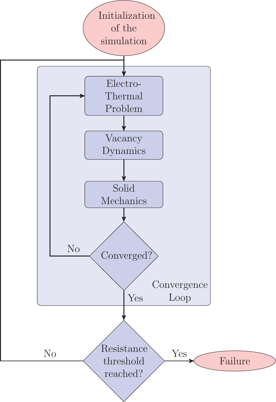
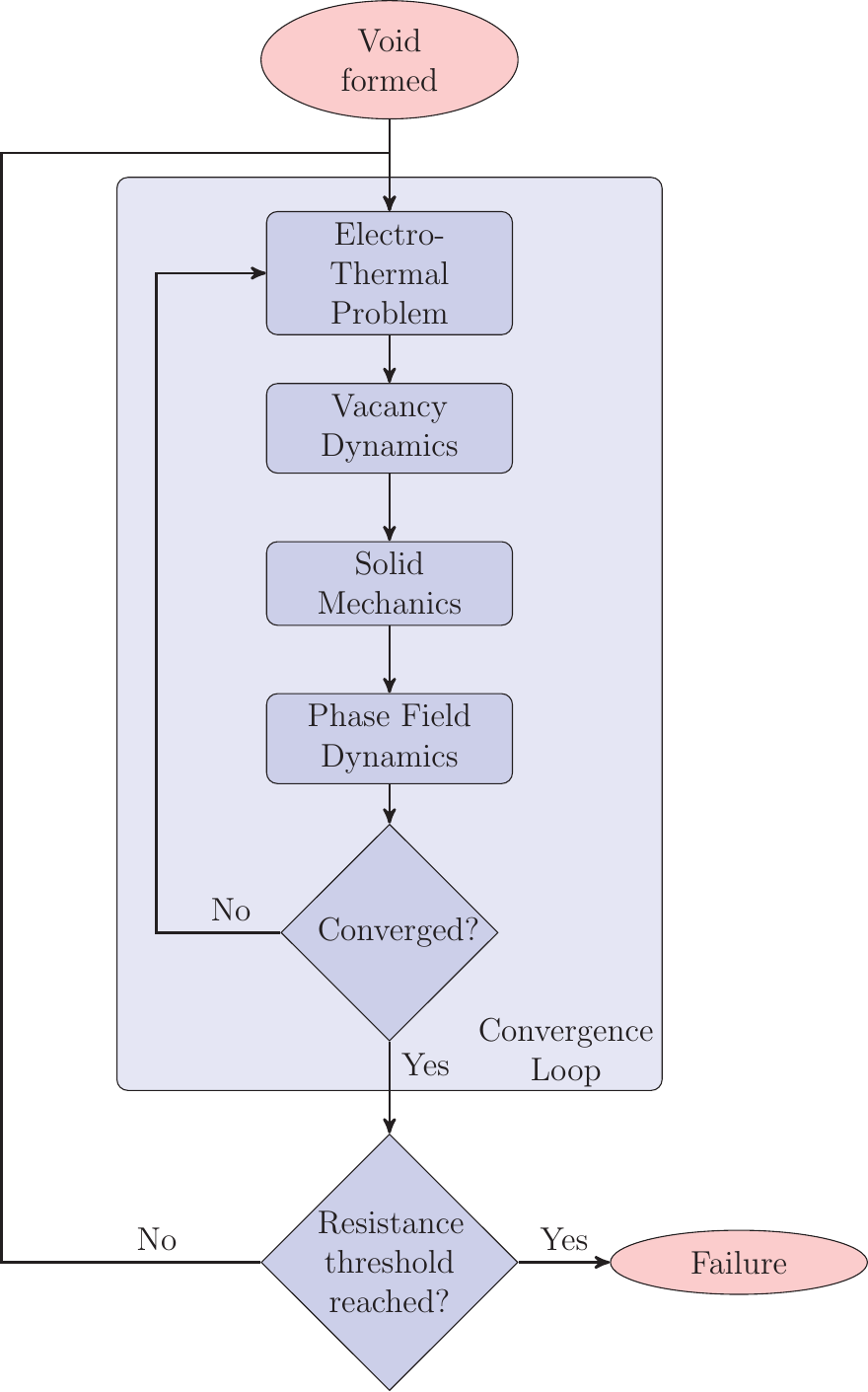
Figure 4.7.: Flowchart of the EM induced void simulation in COMSOL.
4.3.4 Time Stepping
COMSOL offers two methods to compute the solution. The first method called ”Fully Coupled” generates the matrices  and
and  of (4.27) where all differential equations are included at once. These
matrices depend on the solution vector (e.g. the coupling of the vacancy flux and the stress equations) and therefore, first (4.27) is solved where and
of (4.27) where all differential equations are included at once. These
matrices depend on the solution vector (e.g. the coupling of the vacancy flux and the stress equations) and therefore, first (4.27) is solved where and  is retrieved from the old solution vectors.
This step is followed by a regeneration of the matricies using and calculated from the new solution vector
and solving again.
is retrieved from the old solution vectors.
This step is followed by a regeneration of the matricies using and calculated from the new solution vector
and solving again.
These steps are repeated untill convergence is reached. The simulation is terminated under user chosen conditions (e.g. maximum step number), if the problem does not converge. After the solution has converged, the next time step is
computed. The time step size depends on various conditions (e.g. step size to the next chosen output time).
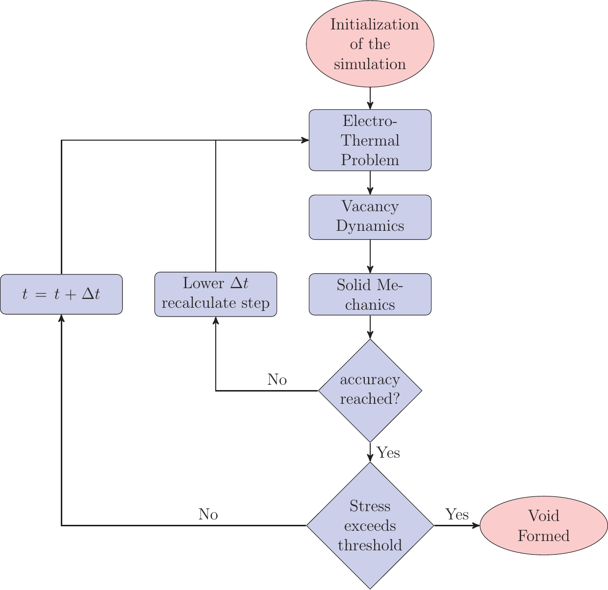
The second method called “Segregated Step” generates the matrices and in (4.27) for every system separately and calculates the solutions
sequentially. The number and the included differential equations of the systems can by chosen by the user. For EM without void modeling the sequence is depicted in Figure 4.6 and for EM modeling with void modeling in
Figure 4.7. This method is the method of choice as the Fully Coupled” method often needs too much memory, since the size of the matrices grows with second order of the number of mesh points.
Previous: 4.2 Implementation in FEDOS Top: 4 Numerical Implementation Next: 5 Results and Discussion