« PreviousUpNext »Contents
Previous: 2 Physics Top: 2 Physics Next: 3 Models
2.2 Quantum Mechanical Electromigration Description
The force due to EM is modeled in continuum mechanical problems as described above by

where the  is called effective valence or effective charge. The EM induced force on an atomic
scale was theoretically studied by Huntington et al. [64]. They used some simplifications, such as the defects are decoupled from the lattice, the electrons are scattered by atoms only, and the creation or annihilation of phonons is
neglected. Under these assumptions the
is called effective valence or effective charge. The EM induced force on an atomic
scale was theoretically studied by Huntington et al. [64]. They used some simplifications, such as the defects are decoupled from the lattice, the electrons are scattered by atoms only, and the creation or annihilation of phonons is
neglected. Under these assumptions the  -directional momentum transferred from the scattered electrons to the defects per time
is given by
-directional momentum transferred from the scattered electrons to the defects per time
is given by

where  is the distribution function of the electrons
and
is the distribution function of the electrons
and  is the transition probability
per unit time of an electron in state
is the transition probability
per unit time of an electron in state  to jump into state
  By separating the two energies’ differentiation into two integrals, interchanging
the primed and the unprimed variables of the second integration, and employing the substitution
By separating the two energies’ differentiation into two integrals, interchanging
the primed and the unprimed variables of the second integration, and employing the substitution

equation (2.21) can be written in the form

where  is the relaxation time of the electrons. As a
common assumption for metals, the relaxation time is taken to be constant over all states
is the relaxation time of the electrons. As a
common assumption for metals, the relaxation time is taken to be constant over all states  describes the electron
distribution at equilibrium and integrates to zero. The current density in the -direction can be expressed by [3, 78]
describes the electron
distribution at equilibrium and integrates to zero. The current density in the -direction can be expressed by [3, 78]

By comparison of (2.21) and (2.24) the relation

is obtained. With the density of defects  , the density of the conducting electrons
  and the contribution of the defects to the resistivity
 the force can
be expressed by
the force can
be expressed by

where the density of the conducting electrons is substituted by  , where
  is the density of the lattice atoms, and
  is the number of conducting electrons per lattice atom. For an ion at a saddle point
between two vacant position the interaction of the ion and the conducting electron is the strongest, whereas the interaction at lattice points is the weakest. On the way from one lattice point to an other the interaction varies and as
this position dependent interaction is not known, Huntington et al. [64] chose a sinusoidal form leading to
is the number of conducting electrons per lattice atom. For an ion at a saddle point
between two vacant position the interaction of the ion and the conducting electron is the strongest, whereas the interaction at lattice points is the weakest. On the way from one lattice point to an other the interaction varies and as
this position dependent interaction is not known, Huntington et al. [64] chose a sinusoidal form leading to

where  is the jump distance, and
  is the maximum force. For a jump path
 with an angle
  between the path and the force , the energy required for a jump can be
calculated by
between the path and the force , the energy required for a jump can be
calculated by

The net flow of atoms due to EM in the current direction is the sum of the probabilities of jumps (along the paths j) times the jump length in the current direction [78].

 is the atomic vibration frequency,
  the concentration of the ions in the metal, and
  the saddle point energy including the formation energy and the motion energy of
vacancies. This equation can be linearized and rewritten to
the saddle point energy including the formation energy and the motion energy of
vacancies. This equation can be linearized and rewritten to

with  being the diffusion coefficient.

The resulting equation (2.30) differs form the Nernst-Einstein relation by the factor 2 in the denominator, which is the average of the chosen position dependent interaction of the conducting electrons and the ions on their path from one lattice point to an other. In addition to the force due to the electron wind also the force due to the electric potential gradient has to be included, leading to the effective charge

and to the effective valence Using the Einstein relation for field assisted diffusion in a potential the drift
velocity can be expressed by [94]

This was the first quantum mechanical expression of the EM induced ion velocity. Within the ballistic model [96] it was shown that there is a linear relation between the EM induced flux and the current density.
For a quantum mechanical force calculation another equation was developed and widely used, based on the scattering states of the conducting electrons [15, 117, 124, 132, 128] obtained from the linear response theory of Kubo [84],
![(2.34) \{begin}{gather} \b {F}_{\mathrm {w}\mathrm {i}\mathrm {n}\mathrm {d}}=\displaystyle \frac {e\Omega }{4\pi ^{3}}\bigg [\iint \limits _{\mathrm
{FS}}\frac {\mathrm {d}^{2}\b {k}}{|\nabla E_{\b {k}}|}\tau _{E_{\b {k}}}\b {v}_{\mathrm {F}}(\b {k})\iiint \psi _{\b {k}}^{*}(r)\nabla _{\b {R}}V(|\b {R}-\b {r}|)\psi _{\b {k}}(\b {r})\mathrm {d}^{3}\b
{r}\bigg ] \cdot {\it \b {E}}. \{end}{gather}](lateximages/lateximage-190.svg)
The considered atom is located at position  and
and  is the effective one-electron
potential.
is the effective one-electron
potential.  is the electric field,
  is the volume of the unit cell,
  is the relaxation time of the scattered
electron,
is the relaxation time of the scattered
electron,  is the -dependent Fermi velocity, and
  is the wave function of the electron,
which can be calculated with the Schröedinger equation [37]
is the wave function of the electron,
which can be calculated with the Schröedinger equation [37]

In (2.34) the first part on the right hand side has the meaning of the effective charge, has the form of a tensor of second order, and reflects the possible dependence of the crystal orientation on the current direction of the EM force especially for non-cubic crystal metals (e.g. zinc) [59]. For periodic structures the integral (2.34) is always equal 0. The reason is the symmetry of the wave functions regarding the crystal wave vector

making the result of the integration over space an even function in due to the fact that the potential is a real valued function,

Furthermore, the Fermi velocity is an odd function in leading to a vanishing result of the integration over the Fermi sphere. This causes
the necessity of calculations of nonperiodic problems. For bulk materials the calculations were performed using the pseudo potential and the KKR method [129, 130, 131, 144, 145].  et al. [15, 111, 112] showed how a calculation for a
single adatom can be carried out by employing the LKKR method [97, 98]. They used the muffin-tin approximation by confining the atomic potential to non-overlapping spheres with a constant interstitial potential [101]. The
advantage of this method is the simplicity and the computational economy payed by an insufficient description of valence electron potentials in covalent open structures [147] compared to full potential calculations [105] The electron
wave function was defined by
et al. [15, 111, 112] showed how a calculation for a
single adatom can be carried out by employing the LKKR method [97, 98]. They used the muffin-tin approximation by confining the atomic potential to non-overlapping spheres with a constant interstitial potential [101]. The
advantage of this method is the simplicity and the computational economy payed by an insufficient description of valence electron potentials in covalent open structures [147] compared to full potential calculations [105] The electron
wave function was defined by

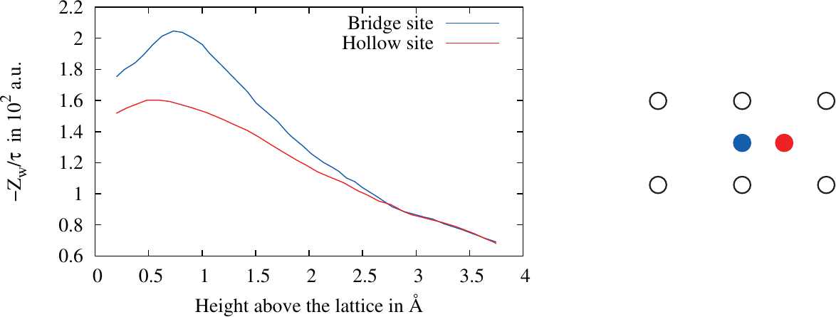
Figure 2.1.: The dependence of the effective valence on the distance of an adatom to a semi-infinite metal surface for two different location above the crystal lattice shown on the right [15].  is the time scale of relaxation of the electronic charge density.
where  is a spherical harmonic [150],
  is the coefficient from the spherical
wave expansion, evaluated by the LKKR calculation, and
is the coefficient from the spherical
wave expansion, evaluated by the LKKR calculation, and  is the spherical solution of the
Schrödinger equation [141], which can be expressed as
is the spherical solution of the
Schrödinger equation [141], which can be expressed as

Here  is a spherical Bessel
function [150],
is a spherical Bessel
function [150],  is the spherical Henkel function [150] of
the first kind, and
is the spherical Henkel function [150] of
the first kind, and  characterizes the scattering phase
shift of each atom. The results show that the effective valance of an adatom is strongly dependent on the height of the atom relative to the metal surface (c.f. Figure 2.1). This dependence is quite well described by a simple ballistic
model, if the reduced electron density relative to the bulk is taken into account [15]. This calculation was extended to islands of adatoms on a substrate modeled by the jellium model showing that the distance to islands has a huge
impact on the effective valance of single adatoms [113].
characterizes the scattering phase
shift of each atom. The results show that the effective valance of an adatom is strongly dependent on the height of the atom relative to the metal surface (c.f. Figure 2.1). This dependence is quite well described by a simple ballistic
model, if the reduced electron density relative to the bulk is taken into account [15]. This calculation was extended to islands of adatoms on a substrate modeled by the jellium model showing that the distance to islands has a huge
impact on the effective valance of single adatoms [113].
Previous: 2 Physics Top: 2 Physics Next: 3 Models