[
Home ]
[
Home ]
[
Home ]
This high-performance C++ library uses the HRLE structure discussed in the previous section to store a LS surface and provides all the necessary algorithms to initialise the surface with a geometry, manipulate the LS values according to a velocity field, analyse features of the surface, and convert the LS to other material representations commonly used in device simulators. It therefore provides all the necessary tools to conduct topography simulations with level set surfaces and provides meshing algorithms to convert these results to be compatible with a device simulator. All algorithms are optimised for the HRLE data structure and thus provide optimal computational efficiency operating on the stored data by moving over all data sequentially and performing all computations in one traversal of the data structure. This library does not include volume information and can thus only be seen as a topography simulation library. However, it forms the basis for the process simulator ViennaPS by providing an accurate description of material interfaces and their evolution over time.
Each surface is described by an instance of the class lsDomain which contains all the necessary information about the simulation domain, including the extent and boundary conditions of the simulation space, and the spacing and orientation of the grid. The sparse-field level set values themselves are stored inside the HRLE structure provided by ViennaHRLE within the lsDomain.
All algorithms are given an instance of lsDomain and operate on the data of this object once they are executed with a call to the algorithm member function apply(). This allows for all properties of algorithms to be initialised without data necessarily being available, followed by the execution of algorithms at a later point, when the data in lsDomain is available for manipulation.
In order to easily distinguish between algorithms and data, all classes holding data are named using nouns, while algorithms operating on data are named as verbs.
In order to quickly generate initial geometries for topography simulations, ViennaLS provides the algorithm lsMakeGeometry to fill a LS with one of four simple shapes:
1. Sphere
2. Plane
3. Box
4. Cylinder
Only the surface of the sphere is generated directly in the LS due to its simplicity, while all other shapes are generated by first creating a triangulated mesh of the shape, translating, and rotating it as necessary, and converting it to a LS representation using the conversion algorithm described in Section 4.2.3.
Once a shape has been generated, it is stored in an lsDomain object, which can be combined with other shapes using Boolean operations, as described in Section 2.3.2.4. For these operations, ViennaLS uses the efficient implementation presented in [169]. The class lsBooleanOperation requires the user to pass a comparator function which takes the LS value from two lsDomain objects at the same point in space. This comparator should then return the LS value for the final surface at this point in space. For convenience, the most commonly used operations, presented in Section 2.3.2.4, are already implemented and can be used directly.
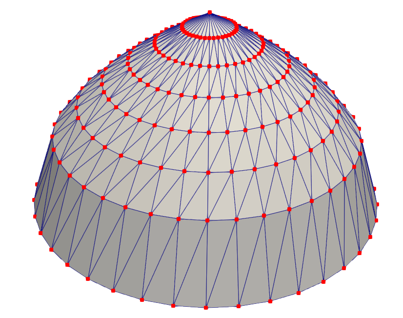
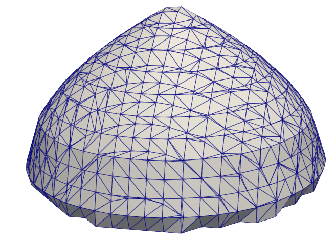
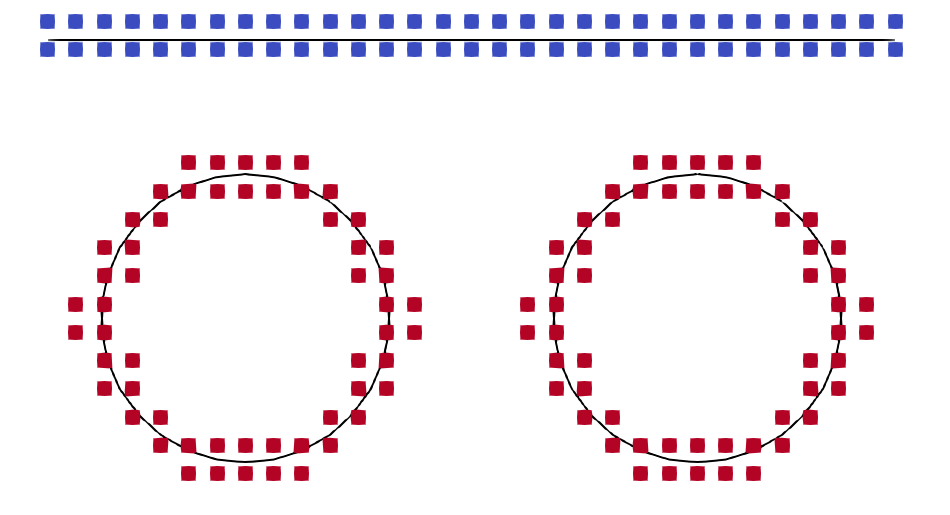
For the generation of more complex, user defined shapes, ViennaLS also offers custom geometries to be created using lsMakeGeometry. This is done by passing a point cloud to the algorithm, which will be converted to a convex hull surface mesh using the gift wrapping algorithm described in [171]. Therefore, more complex shapes, such as the rounded cone shown in Fig. 4.4a, can be created straight-forwardly. The red points shown in the figure are passed to the convex hull algorithm and converted to a triangulated surface mesh with the triangle edges shown in blue. This mesh is guaranteed to be closed, but does not necessarily satisfy other quality criteria, such as equal area triangles or equal edge lengths. However, the algorithm converting this mesh to a LS representation is robust to such meshes and only requires that the mesh is closed, meaning there are no edges which are not part of two triangles. Another restriction is that the resulting mesh is always convex, so in order to generate concave features, several convex structures must be combined using Boolean operations.
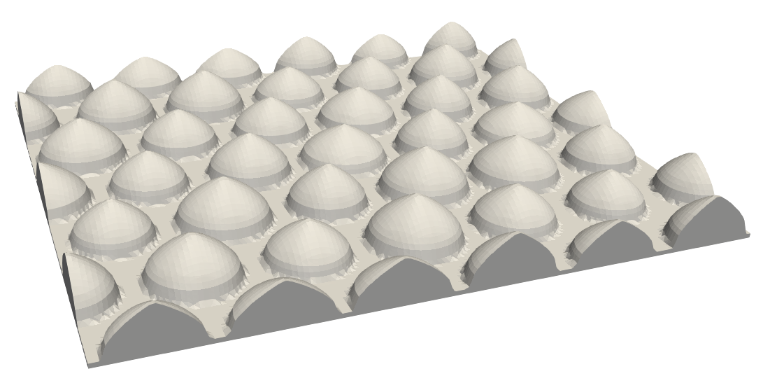
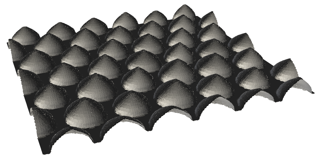
The resulting LS can be combined easily with other LSs using Boolean operations to produce large structures, such as the cone-shaped patterned sapphire substrates [172, 173] shown in Fig. 4.4b, used for enhancing the light extraction efficiency of light-emitting diodes [174]. Large and complex structures can be generated efficiently and straight-forwardly in the ViennaLS library due to the efficient algorithms for Boolean operations in the LS.
(b) Cone-shaped patterned sapphire substrate created by combining numerous level sets, each describing one cone. A final Boolean operation with a plane LS surface results in the final substrate.
Figure 4.4: Creation of a complex patterned substrate by (a) creating the convex hull of a point cloud to generate a cone and (b) combining numerous different cones with a plane surface using Boolean operations.
The ViennaLS library offers algorithms for converting several different explicit surface representations to a sparse-field LS. All conversions follow the same general workflow. First, the explicit material is converted to a line-segmentation in two-dimensional (2D) or triangulation in three-dimensional (3D). Then the sparse-field LS values are found using a closest point transformation and are lexicographically sorted. Finally, the list of sorted points is inserted into the HRLE structure using the efficient initialisation described in Section 4.1.2. If the material interfaces are already given as line-segmented or triangulated surface meshes, they can be converted directly using the algorithm described in the following section.
This type of explicit surface representation only describes material interfaces using line-segments or triangles, referred to as mesh cells. Therefore, the LS value at each grid point \(\vec {g}\) is given by:
\( \seteqsection {4} \)
\begin{equation} \phi (\vec {g}) = \pm \min || \vec {g} - \vec {x}_{s, g} ||_1 \quad , \end{equation}
where \(\vec {x}_{s, g}\) is a point which lies on the explicit surface as well as on a grid line of the LS grid. Only surface points which lie on a grid line are considered, since a Manhattan normalisation is used in the sparse-field method as described in Section 2.3.2.2. Therefore, in order to identify the LS values for the set of active points of the level set, each mesh cell is considered separately. For each cell, intersecting grid lines are identified and the LS values are set for all active grid points satisfying \(|\phi (\vec {g})| \leq 1.0\). If a grid point has already been set using an earlier mesh cell, the smaller absolute value of the two is chosen for the grid point. Once all relevant grid points have been set using all mesh cells, the point list is sorted and used to initialise the HRLE data structure. The algorithm currently implemented in ViennaLS is an adaptation of the closest point transformation algorithm described in more detail in [169].
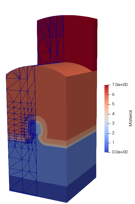
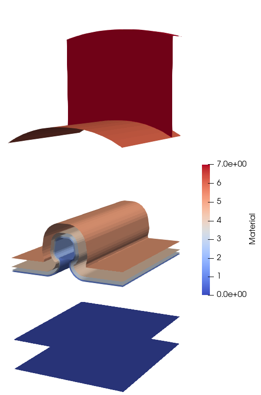
ViennaLS also supports the creation of level sets from triangle meshes in 2D and tetrahedral meshes in 3D. Each cell therefore represents a small volume of a certain material which is denoted by a material identifier for each cell in the mesh. In order to convert these types of meshes to LSs, they are first converted to several surface meshes, one for each distinct material. Each cell is first deconstructed into its surface representation, namely triangles into three line-segments and tetrahedrons into four triangles. These surface elements are then stored in a sorted container and if two surface elements are identical, i.e. contain the exact same nodes, but have opposite normals, they are removed from the list. For volume meshes, containing several materials, surface elements are only removed if the identical but opposite element has a material ID lower than the currently considered one. This automatically results in a surface mesh for each material, with the surfaces automatically following the layer wrapping approach required for the multi-material LS representation described in Section 2.3.2.5, as shown in Fig. 4.5. Finally, each surface is transformed to one LS using the closest point transform described in Section 4.2.3.1.
Figure 4.5: Conversion of a tetrahedral volume mesh into several surface meshes representing the future LS surfaces, respecting the layer wrapping strategy of Section 2.3.2.5.
It is often necessary to obtain an explicit representation of a surface for tasks such as visualisation [175], device simulation [176], or transport modelling using Monte Carlo ray tracing [177]. Therefore, the ViennaLS library allows for the conversion to several different types of explicit surfaces. In the following, each supported explicit representation is discussed in detail, including the required conversion algorithms and the most common applications for these representations in the context of microelectronic simulations are highlighted.
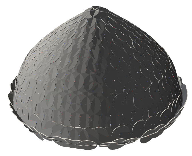
The most efficient way to extract an explicit surface from the LS grid is to shift all active points in the surface normal direction by the distance given by the LS value, as described in Section 2.3.2.3 and Eq. (2.15). This results in a point cloud of the explicit surface described by the level set. As discussed in Section 3.2.3.3, this type of mesh can be used to model molecular transport if a disc is centred at each point of this mesh, hence its name. The radius of the discs needs to be chosen carefully, so there are no holes in the mesh and the discs do not overlap unnecessarily, leading to large smoothing. The mesh itself does not contain this radius explicitly, but it is set during ray tracing. Fig. 4.6 shows that this type of explicit surface contains self-intersections and overlaps which are usually undesirable. However, for the application of Monte Carlo ray tracing, these properties do not have a major effect and thus can be ignored. The disc normal is set to the surface normal at the point around which it is centred, so that each disc forms a tangential plane to the surface at its centre. As can be seen in Fig. 4.6a, the high curvatures at the bottom of the cone result in the back of discs being exposed. Although this is not a problem for the modelling of molecular transport, it must be considered with great care when designing a ray tracing algorithm.
Generating this type of surface mesh can be performed in a single sweep across the HRLE data structure and is thus highly efficient. The only requirement is that the surface normals are known, in order to shift the grid points onto the explicit surface, as described in Section 2.3.2.3. Therefore, the LS has to be extended to include the necessary values required for the calculation of the surface normals.
(b) The entire substrate shown in Fig. 4.4b exported as a disc mesh, as it would be used for Monte Carlo ray tracing.
Figure 4.6: Disc mesh used predominantly for efficient ray tracing. The mesh itself only contains points in space and the surface normals at these points. The discs are visualised to show that they form a closed surface appropriate for ray tracing.
Traditional ray tracing approaches employ conformal triangulated meshes in order to guarantee the properly normalised counting of surface ray intersections [178]. Therefore, triangulated surface meshes can be used for the modelling of molecular transport using Monte Carlo ray tracing, as well as visualisation applications. The marching cubes algorithm [170] is commonly used to generate a line-segmented or triangulated surface from implicit data. It works by considering one grid cell at a time, consisting of \(2^D\) neighbouring LS values. Hence, it is called marching squares in 2D and marching cubes in 3D. Depending on the signs of the grid points and their LS values, different predefined surface elements are chosen from a lookup table. Iterating over all grid cells through which the material interface passes results in a properly extracted explicit surface. Therefore, the algorithm is linear in time with respect to the surface area and thus scales as \(\mathcal {O}(N)\), where \(N\) is the number of LS values. However, since surface elements are added by just considering the current grid cell, the list of meshing nodes has to be checked in order to avoid duplicates. Using an associative data container, such as a hash, for storing the vertices, duplication can be avoided in constant time. The implementation uses the hrleSparseCellIterator discussed in Section 4.1.3 to access the LS values of a grid cell. Vertices are then inserted uniquely into a hash and connected using the lookup table of the marching cubes algorithm. All operations required to extract a triangulated surface can thus be executed in linear time representing the optimal computational efficiency.
Although the triangulation generated by the marching cubes algorithm is sufficient for some visualisation applications, it does not satisfy certain important quality criteria. For example, as shown in Fig. 4.7a, the triangles describing the cone vary strongly in size and some of them are thin and long, which can lead to catastrophic problems in some numerical algorithms used during device simulation. Hence, the meshes generated using this algorithm are not suitable for subsequent device simulation without additional re-meshing steps.
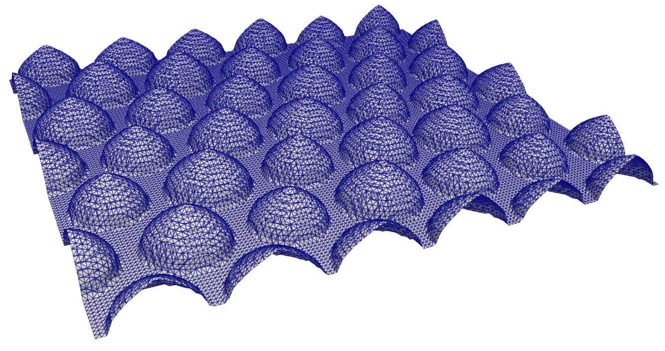
(b) The entire substrate shown in Fig. 4.4b converted from its LS representation to a triangulated surface mesh.
Figure 4.7: The marching cubes algorithm creates a conformal triangulation of the implicit data. Nevertheless, it leads to thin and sharp triangles which are unfavourable for certain applications. The edges of the mesh triangles are shown in blue.
In order to enhance the understanding of a process and its effects on the simulated structures, it might sometimes be necessary to analyse the surface and its exact geometry. Due to the properties of the LS, certain types of analysis can be carried out efficiently and provide useful functionality for automation of process calibration or the efficient realisation of process emulation models. This section discusses the tools that the ViennaLS library provides for the analysis of the geometries represented by the LS.
When dealing with complex surfaces, it is often useful to investigate how many disjoint regions of the surface are present in the simulation domain. If two defined grid points are connected by any number of direct first neighbours, they are part of the same region or component. If this is not possible because there are undefined grid points between these points, they are not connected and thus belong to two separate regions of the surface. In semiconductor process simulations, disjointed material regions usually mean that there is a void somewhere inside a material or that there is a material region which was separated from the substrate. In order to identify such material regions, the HRLE structure is traversed once and the connectivity information is built for every run as described in [169]. This connectivity information is represented by a component ID for each run, denoting to which surface region the respective grid point belongs. During one traversal of the HRLE structure using the hrleSparseStarIterator (see Section 4.1.3) the component IDs are assigned, as described in Algorithm 4.1. Hereby, it is important that every run in the segmentation of the HRLE grid is considered and not just the defined LS values.
Result: information for LS grid
1 highestID = 0;
2 for point in hrleSparseStarIterator do
3 if componentID not defined then
4 if neighbours with sgn(neighbour) = sgn(point) then
5 if 1 distinct neighbourComponentID then
6 componentID = neighbourComponentID;
7 else
8 store connection between different componentIDs;
9 componentID = any neighbourComponentID;
10 end
11 else
12 componentID = highestID;
13 highestID = highestID + 1;
14 end
15 end
16 end
Algorithm 4.1: class="textmd" >Building connectivity information for a LS surface.
As a simple example, the segmentation of a material with two separated voids is shown in Fig. 4.8. Component IDs are assigned based on the neighbouring runs in the HRLE structure. All negative values have the same component ID in this example, as they are all connected through the undefined negative runs U0. Therefore, the disjoint material regions are given by the component IDs of positive values. Intuitively, this makes sense as there is one single material (negative values) and there are several holes denoting lack of material or being outside of the surface (positive values). If all LS values are inverted, then there is one substrate with two additional disjoint material regions. This usually occurs during etching when a geometry is separated and therefore generates two independent material regions. However, numerical inaccuracies can also lead to a small number of stray LS points remaining above the surface after advection. Such grid points are referred to as stray points and can be identified using the connected components algorithm.
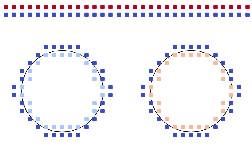
(b) Defined points of the material showing the three component IDs denoting to which section of the surface each point belongs.
Figure 4.8: Using the segmentation of the HRLE structure, connected surface regions can be identified considering first neighbours. This allows for the identification of voids inside a material.
Having identified the connected components, as discussed in the previous section, it is straightforward to identify voids inside or stray points above the material. First the actual substrate must be identified, which can either be the material region with the most points or simply the material region situated in the most negative or positive direction. In the example of Section 4.2.5.1, the latter would be the case and the component ID set at the defined grid point with the most positive \(y\)-value would simply be chosen as the substrate ID. All grid points with differing component IDs must therefore be voids or stray points and can be treated as such.
In this example, only positive points were assigned differing component IDs. Therefore, negative points are not set based on their own component ID but rather based on the component ID of their nearest neighbours. If a negative point has at least one neighbour with the component ID associated with the substrate, it must be part of the substrate. Therefore, another sequential iteration over the HRLE structure is required in order to properly identify different material regions encompassing negative as well as positive values. The results of this identification, conducted on the example structure of the previous section, is shown in Fig. 4.9. When identifying stray points rather than voids, the signs of all of the above considerations must simply be inverted to correctly identify the different surface regions.
For the analysis of simulated structures, the appropriate identification of geometric features is important in several applications, such as denoising [179] and automated image segmentation [180]. In order to identify features, the determination of the exact curvature of the surface is crucial. As described in Section 2.3.2.3, the curvature of a surface described by a LS can be calculated directly without conversion to other surface representations. The curvature for the Stanford bunny test model is shown in Fig. 4.10 for the two types of curvature in 3D.
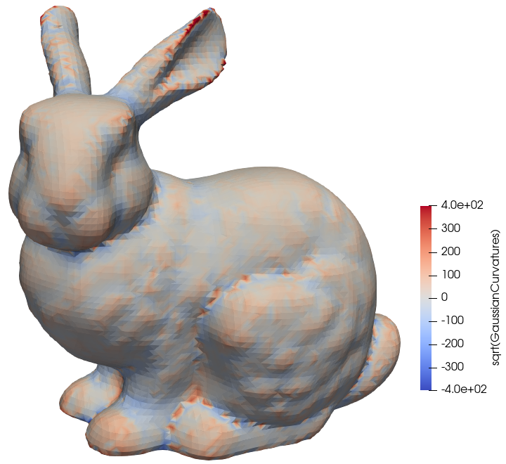
(b) Square root of the Gaussian curvature for the Stanford bunny LS with the original sign of the curvature.
Figure 4.10: Curvature calculated directly in the LS for all defined values of the Stanford bunny geometry. The root of the absolute Gaussian curvature is shown in (b) to compare to the mean curvature in (a), where a negative sign denotes concave curvature.
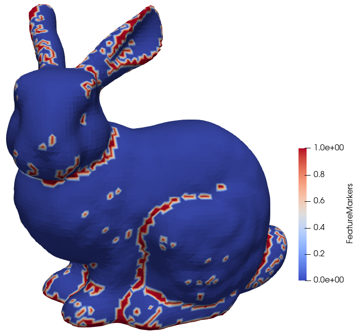
In the simplest case, these curvature values can be used directly for the detection of features. If the curvature exceeds a certain threshold value, the point of the surface is considered a feature. In 3D, only the mean curvature is used to identify features at first. However, the mean curvature may be zero at saddle points or other minimal surfaces, since the two principal curvatures carry opposite signs and may cancel. Therefore, when the mean curvature is below the threshold curvature for features, the Gaussian curvature is evaluated to test if the current point is a minimal surface and thus does in fact represent a feature. As only one threshold is set, it is compared to the square root of the absolute value of the Gaussian curvature, as the latter is equivalent to the square of the principal curvature on minimal surfaces.
This simple scheme for detecting features of the surface already leads to satisfactory results, as shown in Fig. 4.11. Features are highlighted in red and essentially form a binary cut off around a certain curvature value. Points of the surface which are part of a feature can thus be used for subsequent analysis of the structure.
Iterative advection can be implemented very efficiently using the HRLE structure, since all LS values are stored contiguously in memory. The implementation of the iterative advection algorithm consists of three main steps:
1. Calculating the surface velocity
2. Updating LS values
3. Rebuilding a valid sparse field LS
In the first step, the necessary change \(\Delta \phi (\vec {g})\) in the LS value at the grid point \(\vec {g}\) is calculated using one of the numerical integration schemes presented in Section 2.4.2. These values are then used in the second step to find the maximum time step which can be taken without violating the Courant-Friedrichs-Lewy (CFL) condition. The product of the time step and the change in LS value is then applied to all active LS values. Finally, in the third step, grid points are inserted, deleted, or adjusted in order to form a valid sparse field LS again.
In the following, each of these steps will be discussed in depth, highlighting implementation details and computational considerations.
The way in which the surface should move is usually captured in a vector velocity field \(\vec {V}(\vec {g})\). Using an appropriate numerical scheme, this velocity field must be converted to the change in LS value \(\Delta \phi (\vec {g})\) which should be applied at the grid point \(\vec {g}\). This change is equivalent to the Hamiltonian \(\hat {H}\) of the numerical LS equation, presented in Section 2.4.2:
\( \seteqsection {4} \) \( \seteqnumber {2} \)
\begin{equation} \phi (\vec {x}, t + \Delta t) = \phi (\vec {x}, t) - \Delta t~ \hat {H}(\phi (\vec {x}, t), V(\vec {x}, t)) \quad . \tag {\ref {eq::time_discretisation} revisited} \end{equation}
If there is only one LS surface this step is quite straight-forward, as the numerical integration scheme will return the correct value and the LS can simply be updated. However, if multiple materials are present, further considerations are necessary.
Multiple Materials
Using the layer wrapping approach for multiple materials, presented in Section 2.3.2.5, the current material at \(\vec {g}\) has to be identified first. In the presented
implementation, several lsDomain objects are passed to the advection algorithm in the wrapping order. The material ID denoting which LS represents which material in the simulation domain, is simply the array index
to the respective LS. Therefore, a LS with a higher material ID must wrap all LSs with lower material IDs. Due to the way in which the layers are wrapped using Boolean operations, the material present at the grid point \(\vec
{g}\) is described by the LS with the lowest value at this point. Hence, the correct material is found using the following algorithm:
Result: ID of current point \(\vec {g}\)
1 materialID = maxID;
2 i = 0;
3 while i \(<\) maxID do
4 if \(\phi _i(\vec {g}) \leq \phi _{maxID}(\vec {g})\) then
5 materialID = i;
6 break;
7 end
8 i = i + 1
9 end
Algorithm 4.2: class="textmd" >Identification of the material at the grid point \(\vec {g}\) from an array of LSs.
Once the correct material has been identified for each active grid point, the velocity field is constructed using the material information.
Iterative advection can be computationally expensive, due to the numerical derivatives which need to be solved in order to find a solution to the LS equation. Therefore, when advecting several materials, only the top most layer which encompasses all other LSs is advected. This is enough for a deposition process, since a new material is simply added and the initial materials do not change. Hence, advecting only the top LS is enough to describe the physical process.
However, when etching a material or when growing a material around a feature, further considerations are necessary in order to encompass the evolution of several LSs. In this discussion, we will consider the etching of a material around a mask. First, when advecting a material which is masked in certain areas, the top surface can only move to the mask and not further. Therefore, when the top layer would move inside the mask material, it must not be advected further. The simplest way to realise this is to find the LS value of the layer below and to use it to set the advected LS value, in case the top surface would advect further. However, the lower layer might also have a non-zero etch rate if the mask is worn away by the etch process. In this case, the new value for the advected level set \(\phi (t + \Delta t)\) must be found by calculating the Hamiltonian for the top layer \(\hat {H}_0\) and applying it for the time \(\Delta t_0\) until the lower surface is reached. The time \(\Delta t_0\) is found by dividing the difference in level set value of the top and bottom layer by the Hamiltonian of the top layer. From then on, the Hamiltonian \(\hat {H}_1\) for the material below is found and applied until the maximum time \(\Delta t\) for this time step is reached, usually determined by the CFL number. Therefore, the change in LS value is given by:
\( \seteqsection {4} \) \( \seteqnumber {2} \)
\begin{equation} \Delta \phi = \hat {H}_0(V, t) \Delta t_0 + \hat {H}_1(V, t) \Delta t_1 \quad \text {where} \quad \Delta t = \Delta t_0 + \Delta t_1 \end{equation}
An algorithm using the above approach for any number of materials is presented in Algorithm 4.3. Using this approach the different rates for each material can be represented appropriately although only the top LS surface is advected.
Result: in LS value \(\Delta \phi \)
1 cflNumber = 0.5;
2 topIndex = number of LSs - 1;
3 i = topIndex;
4 \(\Delta \phi \) = 0;
5 for i \(>=\) 0 do
6 calculate \(\hat {H}_i\);
7 diff = \(\phi _{i-1}(t)\) - \(\phi _i(t)\);
8 if diff \(\leq \) cflNumber then
9 \(\Delta t_i\) = cflNumber - \(\sum _{j=i+1}^{topIndex} \Delta t_j\);
10 else
11 \(\Delta t_i\) = diff / \(\hat {H}_i\);
12 end
13 \(\Delta \phi \) = \(\Delta \phi \) + \(\hat {H}_i\) \(\Delta t_i\);
14 i = i - 1
15 end
Algorithm 4.3: class="textmd" >Algorithm for the change in LS value for a grid point close to several material interfaces.
Once the above algorithm has concluded for all active grid points, the LSs which were not advected are adjusted by applying a Boolean intersection operation. This means that a material which was removed during the advection of the top LS is also removed for all other level sets. Hence, a set of correctly wrapped LSs is created, including the specific etch rates of all materials.
The CFL condition given in Eq. (2.35) governs how far a sparse field LS can be moved robustly without encountering numerical instabilities, and may be rewritten as:
\( \seteqsection {4} \) \( \seteqnumber {3} \)
\begin{equation} \max _{\text {all}~\vec {g}} | \Delta \phi (\vec {g}) \Delta t | \leq 0.5 \quad . \end{equation}
Since \(\Delta \phi (\vec {g})\) is already given from the previous step, the maximum permitted time step \(\Delta t\) has to be chosen so that the above condition is satisfied for all points \(\vec {g}\). Since the time step is defined globally, it must be the same and therefore the smallest time step must be chosen for the entire simulation domain:
\( \seteqsection {4} \) \( \seteqnumber {4} \)
\begin{equation} \Delta t = \min _{\text {all}~\vec {g}} | 0.5 / \Delta \phi (\vec {g}) | \end{equation}
The new LS values at each grid point are then set as the product \(\Delta \phi (\vec {g}) \Delta t\), which can be carried out highly efficiently as all defined LS values are stored contiguously in memory using the HRLE data structure.
In the previous step, each LS value may have been changed by a maximum of \(\pm 0.5\), meaning that some grid points may not be a part of the \(\mathcal {L}_0\) layer anymore and must therefore be removed, while other grid points may have moved into the \(\mathcal {L}_0\) layer. In order to generate a valid sparse field LS, three rebuilding steps are required:
1. Add grid points which have previously not been in \(\mathcal {L}_0\)
and now satisfy \(|\phi (\vec {g})| \leq 0.5\)
2. Remove grid points which were part of \(\mathcal {L}_0\)
and are not active points anymore
3. Renormalise two oppositely signed neighbours
if both have values larger than \(0.5\)
The last step is not part of the original algorithm and was proposed in [169] in order to avoid invalid LSs for diverging velocity fields. If this step was not considered, two grid points of opposite signs with the surface passing between them could be advected in such a way that neither was active anymore. Although this is only possible if the negative one was reduced and the positive one increased, there is no general limitation on the velocity field disallowing such movement. Hence they could both be removed, although the surface passes between them. In order to avoid this problematic outcome, this third step was introduced, essentially redefining their values so that they are active points again.
All of the above steps can be carried out simultaneously by iterating over the HRLE structure once. During this iteration, a new data structure is built, so the old LS data stays intact. An algorithm providing the functionality to rebuild the sparse field LS after advection using only first neighbours is provided in Algorithm 4.4.
Result: LS from advected LS
1 newLS = empty LS;
2 for point in hrleConstSparseStarIterator do
3 oldValue = LS value at point;
4 if point is active then
5 if point has oppositely signed neighbour then
6 if neighbour not active then
7 newValue = \(\sign (oldValue) \, 0.5\);
8 else
9 newValue = oldValue;
10 end
11 insert newValue into newLS at point;
12 end
13 else
14 if point has oppositely signed, active neighbour then
15 neigbourValue = LS value of neighbour;
16 if \(oldValue > 0\) and \(|neighbourValue + 1| < 1\) then
17 newValue = neighbourValue + 1;
18 end
19 if \(oldValue < 0\) and \(|neighbourValue - 1| < 1\) then
20 newValue = neighbourValue - 1;
21 end
22 insert newValue into newLS at point;
23 end
24 end
25 end
Algorithm 4.4: class="textmd" >Adding, removing, and updating grid points after advection to form a valid sparse field LS.
After this algorithm has concluded, all grid points with absolute LS values smaller than \(1\) will be defined, and all others undefined. Although this is not the smallest set of LS points required to describe the surface, including points up to unity rather than up to \(0.5\) leads to better surface descriptions in areas of high curvature. Therefore, the smallest possible set of grid points robustly describing the surface is created.
The geometric advection algorithm implemented in the ViennaLS library is an efficient implementation of the algorithm introduced in Section 2.4.3. Two parts of this algorithm are essential for high performance: Identification of candidate points, and identification of contribute points. The former requires fast random access in order to iterate over candidate points in the most efficient manner, while the latter requires the fast identification of close points within a certain distance to the current candidate point. Therefore, the HRLE structure is not well suited for this application, although it can be generated quickly from the set of new LS points resulting from the algorithm.
As described in detail in Section 2.4.3, candidate points are grid points which will be active points in the final LS surface after advection. The simplest approach to finding these points is to check every grid point in the simulation domain, and calculate its final level set value from its specific contribute points. However, this algorithm scales as \(\mathcal {O}(N^D)\), where \(N\) is the number of grid points in each dimension \(D\) of the simulation domain.
Better scaling can be achieved by considering the properties of the LS surface. Since every grid point in the simulation domain contains at least the information regarding whether it is inside or outside of the surface, namely its sign, there cannot be any holes in the surface. Since any surface represented in the LS must be closed, every active point must have at least one neighbour which is also an active point. For added robustness, the set of active points can be extended to LS values up to unity rather than \(0.5\), as described in Section 2.4.3. Therefore, if one candidate point of the final surface can be identified, its LS value can be calculated and its neighbours checked to see which one of them is also an active point. If a neighbour is not an active point of the final LS, it is ignored. If it is an active point, then its neighbours are checked and the above procedure is repeated, as presented in Algorithm 4.5. The algorithm effectively marches over the surface, saving active points and their corresponding LS values in an associative container, such as a hash map. If an active point is found which was calculated previously, it is ignored and therefore treated as a non-active point.
Result: of active points of the new surface
1 pointMap = empty hash map;
2 neighbourSet = empty set;
3 a = first active point;
4 add a to hashMap;
5 add neighbours of a to neighbourSet;
6 while neighbourSet is not empty do
7 c = pop point from neighbourSet;
8 if c is not in hashMap then
9 \(\text {value}\) = find LS value for c;
10 if \(\text {value} < 1.0\) then
11 add c to hashMap;
12 add neighbours of c to neighbourSet;
13 end
14 end
15 end
16 construct new LS from hashMap;
Algorithm 4.5: class="textmd" >Efficiently identify candidate points by marching over the surface by looking at direct neighbours of active points.
The first candidate point required to start the algorithm can be identified by considering any initial surface point, centring the geometric distribution around it, and marching through all grid points within the distribution to find one point with an active value. Therefore, the computational effort to identify the first active point is limited and can thus be ignored for large surfaces. Since every active grid point of the final surface only has to be visited once, the algorithm scales as \(\mathcal {O}(N^{D-1})\), corresponding to optimal complexity.
If the surface consists of several disconnected components, as discussed in Section 4.2.5.1, the above algorithm would only apply to the disconnected region to which the first point belongs. Hence, the algorithm requires the identification of the connected components prior to execution. For each component, an initial point must be found and added to the hashMap in Algorithm 4.5. When all disconnected components contain a starting point, the algorithm can commence as above, taking into account all disconnected components of the LS surface.
In order to identify whether a candidate point is an active point of the final surface, all its corresponding contribute points must be evaluated. An efficient algorithm for the identification of contribute points is described in the next section. In Algorithm 4.5 this algorithm is referred to as finding the LS value of the candidate point c (line 9). The calculated LS value is then used to identify whether the point is active.
Finding the neighbour points of any active point is highly efficient, since by definition, all LS values are defined on a rectilinear grid and thus all neighbours are separated by one grid spacing in all Cartesian directions.
The final LS value of each candidate point is calculated from the set of contribute points, which consists of the points close enough to the current candidate point in order to influence its value. Therefore, contribute points only form a small subset of all initial surface points. The fast identification of this subset of initial points is essential for the improved performance of the algorithm. However, surface points are represented explicitly and therefore are not structured in any particular way. In order to quickly access nearest neighbours, a k-d tree data structure is established by sorting the initial points according to their coordinates. The data structure can be queried for all stored points in the neighbourhood of a passed coordinate, returning an iterator over the range of points close to the passed coordinate. By setting the size of the queried neighbourhood to the bounding box of the geometric advection distribution, the minimum number of contribute points can be used for the algorithm.