[
Home ]
[
Home ]
[
Home ]
In order to describe a semiconductor fabrication process with sufficient accuracy, the most important feature of a simulator is the accurate description of the evolution of material surfaces and interfaces over time. For certain types of processes it might be sufficient to simply describe the final result of the process, while for others the precise physical behaviour of materials over time must be included in order to reach a satisfactory final structure. It is therefore necessary to describe simulated materials and their evolution over time with high accuracies in order to achieve satisfactory results. As with the numerical description of materials, the capabilities and limitations of the simulation strongly depend on the numerical method chosen to solve the evolution of material boundaries over time. Several different methods will be discussed here to solve the general problem of moving a numerical surface representing material interfaces.
The movement of a surface in time is usually described by a vector velocity field \(\vec {V}(\vec {x}_s)\) describing where each point on the surface \(\vec {x}_s\) should move. This velocity field is obtained by physical process models or empirical geometric models which will be discussed in Chapter 5. The general problem of generating the final material \(\mathcal {M}(t = t_\text {final})\) must be solved:
\( \seteqsection {2} \) \( \seteqnumber {29} \)
\begin{equation} \mathcal {M}(t = t_\text {final}) ~\text {given}~ \mathcal {M}(t = t_\text {initial}), \vec {V}(\vec {x}_s, t) ~\text {for}~ t \in [t_\text {initial}, t_\text {final}] \end{equation}
Depending on the specific method employed to generate \(\mathcal {M}(t = t_\text {final})\), \(\vec {V}(\vec {x}_s, t)\) might only be required at specific times or only at \(t_\text {initial}\) and not during the entire time range \([t_\text {initial}, t_\text {final}]\). The aim of the numerical methods presented in the following is to apply this velocity field to the surface as accurately as possible with the highest achievable computational efficiency.
Explicit surfaces are evolved over time by shifting the nodes which define the surface in the direction given by the velocity vector \(\vec {V}(\vec {x}_s, t)\) [84]. The surface elements, usually triangles, still connect the same nodes as before and the final surface is thus complete. However, this can lead to non-physical intersections of surface elements [43]. Such a self-intersection is depicted in Fig. 2.15, where two parts of the same material move towards each other and create an overlap between the surface elements.

(a) Valid explicit surface describing initial material.

(b) Broken surface due to a self-intersection.
Figure 2.15: When the nodes (red) of an explicit surface (black lines) describing a material (green) are moved, the result may include regions of non-physical self-intersections (red). These regions must be repaired using subsequent re-meshing steps requiring substantial computational effort.
In order to overcome such non-physical shapes, self-intersections must be found, which is computationally expensive, since every surface element must be checked. Even after identifying affected surface elements, complex re-meshing algorithms must be carried out in order to resolve the conflicting surface elements and to generate the correct physical structure depicted in Fig. 2.15c.
In addition to self-intersections, moving explicit surface representations results in a changing accuracy of the surface description. As an explicit interface is only defined by the nodes on the surface, moving the surface may result in closely spaced nodes in certain sections and widely spaced surface nodes in other sections of the surface, as shown in Fig. 2.16. The resolution may be high in one region, unnecessarily storing surface nodes which are very close together and thus leading to a memory misuse. Another region of the surface may be described by only a few points, leading to a low resolution and an inaccurate description of the interface. In order to mitigate the effects of the changing density of nodes, the surface must be re-meshed regularly to insert or remove nodes where necessary in order to achieve certain mesh quality criteria, such as equal area triangles or equal edge lengths [85]. Although algorithms exist for this type of problem, they require a substantial amount of computational effort and are thus undesirable for complex 3D simulations.
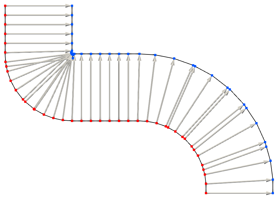
Figure 2.16: Nodes (red), defining the initial material interface (black), are shifted by the surface normals (arrows) to move the surface outwards isotropically as would occur during conformal deposition. The nodes of the final interface (blue) are spaced differently, leading to many overlapping points in areas of concave curvature and widely spaced points in area of convex curvature.
Moving an implicit surface is referred to as advection and is governed by a differential equation called the LS equation
\( \seteqsection {2} \) \( \seteqnumber {30} \)
\begin{equation} \frac {\partial \phi (\vec {x}, t)}{\partial t} + V(\vec {x}, t) ||\nabla \phi (\vec {x}, t)||_2 = 0 \quad , \label {eq::LS_equation} \end{equation}
where \(V(\vec {x}, t)\) is a scalar velocity field denoting the speed of the propagation in the normal direction to the surface. Given \(\vec {V}(\vec {x}, t)\) and surface normal vectors \(\hat {n}(\vec {x})\) calculated with Eq. (2.11), the scalar velocity field is given by
\( \seteqsection {2} \) \( \seteqnumber {31} \)
\begin{equation} V(\vec {x}, t) = \vec {V}(\vec {x}, t) \cdot \hat {n}(\vec {x}) \quad . \label {eq::normalV} \end{equation}
Many process models give an expression for the surface speed already in the normal direction which can then be applied directly.
In order to find \(\mathcal {M}_\text {final}\), Eq. (2.30) must be solved to find \(\phi (\vec {x}, t_\text {final})\). Since the LS equation is a Hamilton-Jacobi type differential equation, numerous numerical schemes are available to solve it, which differ in complexity, performance and assumptions about the velocity function. In order to apply such numerical schemes, Eq. (2.30) is rewritten as
\( \seteqsection {2} \) \( \seteqnumber {32} \)
\begin{equation} \frac {\partial \phi (\vec {x}, t)}{\partial t} + \hat {H}(\phi (\vec {x}, t), V(\vec {x}, t)) = 0 \quad , \label {eq::hamilton_jacobi} \end{equation}
where the Hamiltonian is simply given by \(\hat {H}(\phi (\vec {x}, t), V(\vec {x}, t)) = V(\vec {x}, t) ||\nabla \phi (\vec {x}, t)||_2\).
In order to solve Eq. (2.32), the first step is to discretise time into several time steps of size \(\Delta t\). The solution is then computed iteratively for each time step \(\Delta t\) until \(t_\text {final}\) is reached. One of the simplest numerical schemes to solve a differential equation is the first-order Euler method [86] which requires the Hamiltonian to be evaluated only once per time step. Therefore, the evolution of the LS during one time step is given by
\( \seteqsection {2} \) \( \seteqnumber {33} \)
\begin{equation} \phi (\vec {x}, t + \Delta t) = \phi (\vec {x}, t) - \Delta t~ \hat {H}(\phi (\vec {x}, t), V(\vec {x}, t)) \quad . \label {eq::time_discretisation} \end{equation}
Therefore, the entire change of the surface during one time step is encapsulated in the second term. The new LS value for each point \(\vec {x}\) is calculated by simply subtracting the Hamiltonian from the initial LS value. More complex schemes for the solution in time exist and lead to better results through additional evaluations of the Hamiltonian [87] or higher order approximations [88, 89]. Such complex schemes require more computational effort and thus increased simulation time. However, regardless of the chosen numerical scheme, certain conditions must be met in order to guarantee numeric stability. These will be discussed further in the following sections.
For a full grid level set, the velocity field \(V(\vec {x}, t)\) must be defined in the entire domain in order to solve Eq. (2.30). Since space is discretised, this means that there must be a value \(V(\vec {g}, t)\) for every grid point \(\vec {g}\) in the domain. However, during process simulations, only material interfaces are modelled and thus velocities can only be calculated at the interface itself. Therefore, the surface velocity must be extrapolated to all other grid points.
The speed at which the implicit function should move is generated by considering the closest surface point and using its velocity value [90]. In order to achieve this efficiently, the values for the velocity are propagated from the zero level set outwards, which is referred to as velocity extension [49]. This results in the same numerical problem, as for generating neighbouring level set values discussed in Section 2.3.2.2 [91]. The previously mentioned methods can be employed analogously to the extension of the surface velocities to the domain. In the case of sparse field level sets, this step can be ignored since only the \(\mathcal {L}_0\) layer is used for advection. Only the points closest to the surface are used to describe the implicit function and the velocity field must be defined directly for these grid points, hence there is no need for a velocity extension.
Numerical time integration schemes are used to propagate information from the surface. Due to the time and spatial discretisation of the problem, there is a maximum distance information should propagate in one time step, which is given by the Courant-Friedrichs-Lewy (CFL) condition [92]. For the advection of a LS, this condition limits how much a single LS value is allowed to be changed in a single time step, before all other LS values must be updated in order to guarantee numerical stability. Hence, it sets a maximum distance the surface should be moved for one solution of Eq. (2.30), i.e., one time step. This maximum distance, according to the CFL condition, is given by:
\( \seteqsection {2} \) \( \seteqnumber {34} \)
\begin{equation} \max | \hat {H}(\phi (\vec {g}, t)) \Delta t | = \max |\phi (\vec {g}, t + \Delta t) - \phi (\vec {g}, t)| \leq 1 \quad , \label {eq::CFL_condition} \end{equation}
where the difference in LS values is simply the product of the Hamiltonian and the time step, as defined in Eq. (2.33). Since the difference in \(\phi (\vec {g}, t)\) values must be smaller than 1, effectively the surface must not be moved more than one grid spacing in a single time step in order to guarantee stable numerical solutions.
In the case of sparse-field level sets, only LS values with an absolute value lower than \(0.5\) are stored. If an active point \(\vec {a}\) is advected according to the maximum set by Eq. (2.34), the minimum value the point may have is \(\phi (\vec {a}, t + \Delta t) = 0.5\), while the maximum value is \(1.5\). This means that the surface will no longer be located between this point and one of its neighbours after advection, meaning there will be no valid zero level set layer \(\mathcal {L}_0\). As this layer contains all the information about the surface, a valid LS cannot be formed robustly anymore. Although the \(\mathcal {L}_0\) layer could be reconstructed from neighbouring layers, this may lead to large numerical errors and hence a stricter CFL condition must be chosen for sparse-field level sets [47]. The maximum change in \(\phi (\vec {g}, t)\) during one time step is then given by:
\( \seteqsection {2} \) \( \seteqnumber {35} \)
\begin{equation} \max | \hat {H}(\phi (\vec {g}, t)) \Delta t | = \max |\phi (\vec {g}, t + \Delta t) - \phi (\vec {g}, t)| \leq 0.5 \quad . \label {eq::CFL_condition_sparse} \end{equation}
In practice, this condition is satisfied by reducing the time increment \(\Delta t\) until the change in \(\phi (\vec {g}, t)\) becomes small enough. Therefore, the time integration and the solution to \(\hat {H}\) must be recomputed every time any part of the surface moves by more than half the grid spacing, or more than the predefined CFL condition. The advection must thus be repeated until the simulation time has advanced to the full process time of the simulation fabrication step. Note that Eq. (2.34) or Eq. (2.35) must be satisfied regardless of the numerical scheme chosen for the solution of the LS equation. Therefore, this type of advection must always be conducted by taking multiple time steps, which is why it is referred to as iterative advection.
The change of LS values for a time step depends on the Hamiltonian which is a differential equation in space and must be solved using appropriate spatial schemes. According to the definition in Eq. (2.6), the implicit function is stored on a rectilinear grid with grid points \(\vec {g}\), which can be used to solve \(\hat {H}\). In the following, several numerical schemes used to approximate the Hamiltonian will be discussed.
Upwind schemes are one of the earliest-developed methods to numerically solve hyperbolic partial differential equations (PDEs) [93]. After Engquist and Osher proposed their finite difference numerical scheme for stable and entropy satisfying flow in 1980 [94], Osher and Sethian employed a version of this upwind scheme to solve the LS equation in 1988 [42]. Upwind schemes use one-sided approximations to a PDE based on the direction of flow of information of the system. A simple example is the one-dimensional LS equation
\( \seteqsection {2} \) \( \seteqnumber {36} \)
\begin{equation} \frac {\partial \phi (x, t)}{\partial t} - V(x, t) \frac {\partial \phi (x, t)}{\partial x} = 0 \quad . \label {eq::LS_equation1D} \end{equation}
Depending on the sign of \(V(x, t)\), the surface and thus the information propagates towards positive or negative \(x\). The direction the information is propagating towards is called downwind, while the direction the information coming from is called upwind. In this scheme, the solution is approximated by only considering the information of the initial equation upwind of \(x\) giving this scheme its name.
Using the definition of the forward and backward difference from Eq. (2.12), the numerical derivative \(\partial _x\phi (x, t)\) of the 1D problem in Eq. (2.36) is defined for the upwind scheme as
\( \seteqsection {2} \) \( \seteqnumber {37} \)
\begin{equation} \partial _x^1 \phi (g, t) \approx \left \{ \begin {array}{@{}ll@{}} D_x^-(\phi (g, t)) \quad \text {if} ~\sign (V(g, t)) = \sign (D_x^-(\phi (g, t))) \\ D_x^+(\phi (g, t)) \quad \text {otherwise} \quad , \label {eq::upwind1D} \end {array}\right . \end{equation}
where \(\sign (x)\) is the signum function which returns \(-1\) for negative \(x\) and \(+1\) for positive \(x\). The superscript \(1\) in \(\partial _x^1\) denotes that this is the first order approximation to the partial derivative. Whether the forward finite difference \(D_x^+\) or the backward finite difference \(D_x^-\) is chosen thus depends on both the sign of the scalar velocity field and the sign of the finite differences themselves. This is expected because a change in the sign of finite differences means that the surface is facing in the opposite direction. If this is the case, the direction of the advection and thus the propagation of information is also changed, meaning the other finite difference must be chosen in order to use the upwind side. The definition given here is valid only for the convention that the LS values inside the surface are negative. If the opposite convention is chosen, the forward and backward differences simply need to be exchanged to achieve the correct result.
In dimensions higher than 1, the spatial derivative is given by the \(\ell _2\) norm of all components of the gradient, as defined in Eq. (2.30), and the Hamiltonian is thus
\( \seteqsection {2} \) \( \seteqnumber {38} \)
\begin{equation} \hat {H} \approx V(g, t) \sqrt { \sum _{i=1}^{D} \partial _i \phi (g_i, t)} \quad , \label {eq::hamiltonian} \end{equation}
where \(g_i\) is the \(i^{th}\) component of the grid point coordinate \(\vec {g}\) and \(\partial _i\) is the finite difference in the dimension \(i\) as defined in Eq. (2.37). The result of this numerical scheme is first order accurate in space. If higher precision is needed, the second order scheme can be applied by including an additional term in the numerical derivative:
\( \seteqsection {2} \) \( \seteqnumber {39} \)
\begin{equation} \partial _i^2 \phi (g, t) \approx \left \{ \begin {array}{@{}ll@{}} D_i^-(\phi (g, t)) + \frac {\Delta g}{2} D_i^{–}(\phi (g, t)) \quad \text {if} ~\sign (V(g, t)) = \sign (D_i^-(\phi (g, t))) \\ D_i^+(\phi (g, t)) - \frac {\Delta g}{2} D_i^{++}(\phi (g, t)) \quad \text {otherwise} \quad . \label {eq::upwind1D_2nd} \end {array}\right . \end{equation}
The second order term for the approximation of the derivative is calculated by applying two one-sided numerical differences and choosing the appropriate result
\( \seteqsection {2} \) \( \seteqnumber {40} \)
\begin{equation} D_x^{\pm \pm }(\phi (g, t)) = \zeta \left (D_x^{\pm }\left ( D_x^{\pm }(\phi (g, t)) \right ), D_x^{-}\left ( D_x^{+}(\phi (g, t)) \right ) \right ) \quad , \label {eq::second_order_differential} \end{equation}
where \(\zeta \) is a switch function selecting the correct upwind side using the absolute values of its arguments, the differential approximations:
\( \seteqsection {2} \) \( \seteqnumber {41} \)
\begin{equation} \zeta (a, b) = \left \{ \begin {array}{@{}ll@{}} a \quad \text {if} ~|a| \leq |b|\\ b \quad \text {otherwise} \label {eq::second_order_diff} \end {array}\right . \end{equation}
The final value of the Hamiltonian is then computed in the same way as for the first-order approximation shown in Eq. (2.38).
Non-convex Hamiltonians
Due to the nature of the upwind scheme, stability is only guaranteed for convex Hamiltonians [44]. Convexity of the Hamiltonian is defined as
\( \seteqsection {2} \) \( \seteqnumber {42} \)
\begin{equation} \frac {\partial ^2 \hat {H}}{\partial \phi _i \partial \phi _j} = \frac {\partial ^2 V(\vec {x}, t) ||\nabla \phi (\vec {x}, t)||_2}{\partial \phi _i \partial \phi _j}\geq 0 \quad \text {for all } i, j \quad , \label {eq::convexity} \end{equation}
where \(\phi _i\) is the partial derivative of \(\phi (\vec {x}, t)\) with respect to the spatial coordinate \(i \in \{ 1, ..., D \}\). If the Hamiltonian is non-convex, wave-like properties may distribute through the simulation domain and thus result in unphysical geometries [95].
As discussed in Section 2.3.2.3, the surface normals of the LS are found by evaluating the partial derivatives in all directions. Therefore, surface normal dependent velocity fields may result in non-convex Hamiltonians leading to problematic numerical errors when using upwind schemes [95]. Therefore, the suitability of the Engquist-Osher scheme for the solution of the specific velocity field must be guaranteed by ensuring that the condition in Eq. (2.42) is satisfied for all derivatives \(\partial \phi _i, \partial \phi _j\).
Upwind schemes take one-sided approximations to the Hamiltonian depending on the direction of information propagation. The Lax-Friedrichs scheme uses central differences to obtain the gradient and thus achieves more accurate results than upwind schemes [96]. The numerical derivatives used to solve the Hamiltonian are defined as
\( \seteqsection {2} \) \( \seteqnumber {43} \)
\begin{equation} \partial _i^\pm (\phi (\vec {g}, t)) = D_i^\pm (\phi (g, t)) \mp \frac {\Delta g}{2} D_i^{\pm \pm }(\phi (g, t)) \quad , \end{equation}
where \(D_i^{\pm \pm }\) is the second order term defined in Eq. (2.40). If only the first order approximation is used, this term can be omitted. Using these numerical differences, the Hamiltonian is approximated using
\( \seteqsection {2} \) \( \seteqnumber {44} \)
\begin{equation} \hat {H} \approx V(\vec {g}, t) \sqrt {\sum _{i=1}^{D} \left ( \frac {\partial _i^-(\phi (\vec {g}, t)) + \partial _i^+(\phi (\vec {g}, t))}{2} \right ) ^2} - D_{LF} \quad , \end{equation}
where \(D_{LF}\) is an additional dissipation term defined as
\( \seteqsection {2} \) \( \seteqnumber {45} \)
\begin{equation} D_{LF} = \sum _{i=1}^{D} \alpha _i \left ( \frac {\partial _i^-(\phi (\vec {g}, t)) - \partial _i^+(\phi (\vec {g}, t))}{2} \right ) \quad , \end{equation}
where \(\alpha _i\) are the dissipation coefficients. The numerical dissipation is non-zero in regions of high curvature, i.e. where the LS function changes abruptly. Especially at discontinuities, such as sharp corners of the surface, unphysical oscillations may be introduced into the LS, which are balanced by this dissipation term [97]. In order to achieve robust results, the dissipation coefficients must be chosen correctly. If they are too small, unphysical behaviour is not suppressed and oscillations still occur on the surface. If they are too large, sharp features are smoothed unnecessarily. The correct \(\alpha _i\) values can be chosen by considering that the scheme is stable if it is monotone [98]. This means that the Hamiltonian must have a positive gradient along each direction of change for every point in space. Using the partial derivative \(\phi _i = \partial \phi (x_i, t)/\partial x_i\), several inequalities must be satisfied to ensure a monotone Hamiltonian:
\( \seteqsection {2} \) \( \seteqnumber {46} \)\begin{align} \left | \frac {\partial \hat {H}}{\partial \phi _i} \right | &\leq \alpha _i \quad \text {for $i$} \in \{ 1, ..., D \} \text {, for all $\vec {x}$} \\ \Delta t \left ( \sum _{i=1}^{D} \frac {\alpha _i}{\Delta g} \right ) &\leq 1 \quad \text {for all $\vec {g}$} \end{align} In order to chose appropriate values for the dissipation without unnecessary smoothing, these inequalities can be equated, i.e. choosing the largest possible time step \(\Delta t\) and the smallest allowed values for \(\alpha _i\). Since \(\alpha _i\) is the partial derivative of the Hamiltonian, the inequalities can be expressed as [48]
\( \seteqsection {2} \) \( \seteqnumber {48} \)\begin{align} \alpha _i &= \max _{\text {all $\vec {g}$}} \left | \frac {\partial \hat {H}}{\partial \phi _i} \right | \quad \text {for $i$} \in \{ 1, ..., D \} \\ \Delta t &= \min \left [ \left ( \sum _{i=1}^{D} \frac {\alpha _i}{\Delta g} \right )^{-1} \right ] \end{align} If the scalar velocity field \(V(\vec {x}, t)\) can be expressed analytically, all necessary values can be found straight-forwardly by solving the partial derivatives analytically [95].
Dissipation for Spatially Constant Velocity Fields
Usually, the velocity field is not given analytically, but rather it is defined only on the discretised grid as \(V(\vec {g}, t)\). In this case, the correct values for \(\alpha _i\) must be found numerically. In the simplest case, the
velocity is constant in the simulation domain and the partial derivative of the Hamiltonian is simply
\( \seteqsection {2} \) \( \seteqnumber {50} \)
\begin{equation} \alpha _i = \left | \frac {\partial \hat {H}}{\partial \phi _i} \right | = \left | V(t) \frac {\phi _i}{||\nabla \phi (t)||_2} \right | = \max _{\text {all}~\vec {g}} \left | V(t) n_i(\vec {g}) \right | \quad , \label {eq::lax_friedrichs} \end{equation}
where \(n_i(\vec {g})\) is the ith component of the surface normal vector which, according to Eq. (2.11), can be written as \(\frac {\phi _i}{||\nabla \phi ||_2}\).
Dissipation for Normal Vector Dependent Velocity Fields
If the velocity field does depend on the normal vector of the surface and cannot be expressed analytically, Eq. (2.50) cannot be used. In this case,
the values for \(\alpha _i\) must be generated by solving the partial derivative of the Hamiltonian numerically. For simplicity, the dependency of the velocity field \(V(\vec {n}, t)\) on the normal vector and the time will not be
written explicitly in the following. Since the velocity field is now dependent on \(\phi _i\), the Hamiltonian is differentiated according to the product rule:
\( \seteqsection {2} \) \( \seteqnumber {51} \)
\begin{equation} \frac {\partial \hat {H}}{\partial \phi _i} = \frac {\partial V}{\partial \phi _i} ||\nabla \phi ||_2 + V \frac {\partial ||\nabla \phi ||_2}{\partial \phi _i} \quad , \end{equation}
where the second term is simply the result obtained in Eq. (2.50) for constant velocity fields. The velocity field may depend on all components of the normal vector \(n_j\) and thus on all \(\phi _j\). Therefore, the differential of the velocity field with respect to \(\phi _i\) may be written as
\( \seteqsection {2} \) \( \seteqnumber {52} \)
\begin{equation} \frac {\partial V}{\partial \phi _i} = \sum _{j=1}^{D} \frac {\partial V}{\partial n_j} \frac {\partial n_j}{\partial \phi _i} \quad . \label {eq::velocityDiff} \end{equation}
Differentiating all terms then leads to
\( \seteqsection {2} \) \( \seteqnumber {53} \)
\begin{equation} \frac {\partial V}{\partial \phi _i} = ||\nabla \phi ||_2^{-3} \left [ \frac {\partial V}{\partial n_i} \left ( \sum _{j \neq i} \phi _j^2 \right ) - \sum _{j\neq i}\frac {\partial V}{\partial n_j} \phi _i \phi _j \right ] \quad . \end{equation}
Using the above results, the dissipation can be rewritten as
\( \seteqsection {2} \) \( \seteqnumber {54} \)
\begin{equation} \alpha _i = \left | V n_i + \frac {\partial V}{\partial n_i} \left ( \sum _{j \neq i} \frac {\phi _j^2}{\displaystyle ||\nabla \phi ||_2^2} \right ) - \sum _{j\neq i}\frac {\partial V}{\partial n_j} \frac {\phi _i \phi _j}{\displaystyle ||\nabla \phi ||_2^2} \right | \quad , \end{equation}
where the first term is simply the result for spatially constant V, the second term is the derivative in the \(i\) direction proposed by Montoliu et al. [99] and the third term encompasses cross-directional derivatives as proposed by Toifl et al. [100] within the scope of this work. All terms can be found directly from \(\phi \), except the \(\partial V / \partial n_i\) terms. These must be solved numerically, which can be achieved using a central difference scheme [99]. The derivative is then approximated as
\( \seteqsection {2} \) \( \seteqnumber {55} \)
\begin{equation} \frac {\partial V}{\partial n_i} \approx \frac {V(n_i + \Delta n) - V(n_i - \Delta n)}{2\Delta n} \quad , \end{equation}
where all other components of the normal vector are kept constant. \(\Delta n\) is the finite difference, which is either given by the discretisation of the normal vector values or may be chosen freely. A stable numerical choice is
\( \seteqsection {2} \) \( \seteqnumber {56} \)
\begin{equation} \Delta n = \epsilon ^{\frac {1}{3}} V(\vec {n}, t) \quad , \end{equation}
where \(\epsilon \) is the floating point accuracy of the simulator [101].
Dissipation for General Velocity Fields
A general velocity field may depend on the current time, the surface normal and the spatial coordinate and is thus defined as \(V(t, \vec {n}, \vec {x})\). Due to the additional dependency on location \(\vec {x}\), the derivative
of \(V\), with respect to \(\phi _i\) in Eq. (2.52), must be extended by spatial terms:
\( \seteqsection {2} \) \( \seteqnumber {57} \)
\begin{equation} \frac {\partial V}{\partial \phi _i} = \sum _{j=1}^{D} \left ( \frac {\partial V}{\partial n_j} \frac {\partial n_j}{\partial \phi _i} + \frac {\partial V}{\partial x_j} \frac {\partial x_j}{\partial \phi _i} \right ) \end{equation}
To the best of the authors’ knowledge no general expression for the solution of the second term has been presented to date. However, for certain applications, where the spatial dependence of the velocity field is much smaller than the dependence on the normal vector, the second term may be ignored. In certain types of epitaxial growth, arriving molecules may diffuse along the surface for large distances before reacting with the substrate, meaning that there is no large change of growth rate with distance. This type of growth is, however, strongly dependent on the surface normal, such that most of the dissipation will stem from the normal vector dependence. As \(\partial V / \partial x_j\) is much smaller than \(\partial V / \partial n_j\), the spatial component does not contribute significantly to the dissipation. Hence, ignoring the spatial component may be viable for some simulations, although a general solution incorporating the spatial dependence of \(V\) would certainly be favourable. When there is a spatial dependence, but the velocity does not depend on the surface normal, the Hamiltonian is convex as defined by Eq. (2.42) and the Upwind scheme presented in Section 2.4.2.3 can be used instead.
Stencil-Based Schemes
Using the above definitions for \(\alpha _i\), global dissipation coefficients are chosen based on the maximum value encountered in the entire simulation domain, which is why this technique is referred to as Global Lax-Friedrichs
scheme. However, this may lead to large values of \(\alpha _i\) and thus to unnecessary smoothing in large parts of the surface, as high curvatures might only occur in small regions of the surface.
The gradient of the Hamiltonian is a local property of the implicit function and thus, the Global Lax-Friedrichs scheme overestimates the values for \(\alpha _i\) and therefore leads to high smoothing [102, 103]. In order to reduce this smoothing effect, one may use only the neighbourhood of the current grid point for the calculation of the dissipation. Such a scheme was developed as a part of this work and is referred to as Stencil Local Lax-Friedrichs (SLLF) [96]. The dissipation is then defined as
\( \seteqsection {2} \) \( \seteqnumber {58} \)
\begin{equation} \alpha _i(\vec {g}) = \left | \frac {\partial \hat {H}}{\partial \phi _i} \right |_S = \max _{\vec {g} \in S} \left | V(t) n_i(\vec {g}) \right | \quad , \end{equation}
where \(S\) is the stencil made of the current point and neighbouring points. This method uses a 49-point stencil around the current grid point. However, smaller stencils are possible. For example, the Local Lax-Friedrichs (LLF) scheme proposed in [104] uses only the first neighbours, meaning 9 and 27 grid points in 2D and 3D, respectively. In the extreme case, only the current grid point is used [48], which is referred to as Local Local Lax-Friedrichs (LLLF). While LLLF requires the least computational effort, it usually underestimates the required dissipation coefficient and thus results in unphysical oscillations. LLF achieves satisfactory values for \(\alpha _i\), while keeping the computational requirements at a minimum. Therefore, this scheme is the most appropriate for the advection of general velocity functions \(V(\vec {g}, t)\).
It is important to note that although stencil-based schemes are used to obtain spatially varying dissipation coefficients \(\alpha (\vec {g})\), the size of the time step \(\Delta t\) still must be chosen based on the global \(\alpha _i\) values, since the time step is a global property. Therefore, the correct size of the time step for stencil-based schemes is
\( \seteqsection {2} \) \( \seteqnumber {59} \)
\begin{equation} \Delta t = \min _{\text {all } \vec {g} \in \mathcal {L}_0} \left | \left ( \sum _{i=1}^D \frac {\alpha _i}{\Delta g} \right )^{-1} \right | \quad . \end{equation}
In Section 2.4.2, the evolution of a level set was modelled by considering the surface normal speed and solving the propagation of the surface iteratively. In each iteration, only a small time step can be applied, due to numeric restrictions of the underlying methods used to advance the surface. At most, the zero LS can be moved by half a grid spacing when using the sparse field approach. Hence, when a surface is represented at a high resolution, several hundred time steps might be necessary to advance the surface to its final location. Therefore, moving the interface using iterative advection commonly requires substantial computational effort, while introducing numerical errors [105]. Such errors stem from the approximations of partial derivatives, required to solve the level set equation, as discussed in the previous section.
If the propagation of time does not have to be modelled explicitly, meaning that a geometric relationship between the initial and the final surface is known, there is no need to move the surface in small steps. The resulting geometry can then simply be "drawn" based on this geometric relationship, which is referred to as geometric advection or process emulation [106]. This way, perfectly isotropic deposition can simply be thought of as extending the surface outwards at every point by a constant distance. This method of emulating surface movement was first applied successfully using explicit voxel-based representations [107, 108] similar to those described in Section 2.3.3.2.
Within the scope of this work, the method of emulation was applied to the LS for the first time. Due to the higher resolution of the LS as compared to voxel-based surface representations, better results can be achieved with comparable computational effort. Additionally, this allows geometric advection to be combined with iterative advection to achieve a high flexibility with regard to the modelling capabilities of the implemented simulator. In this section, the underlying geometric advection algorithm, as developed during this work, is presented including considerations for practical applications, as well as fundamental limitations of this approach.
In order to familiarise the reader, the general approach of this method will first be explained using an explicit surface representation. Applying the same strategy to level sets, most algorithmic approaches remain the same and can be applied to the implicit surface.
For voxel-based advection, the initial surface is described as a Cartesian grid of cells, where each cell is filled with an integer denoting which material it contains. Usually, partially filled cells are not permitted [109], since this would strongly increase the complexity of the algorithm and thus lead to increased computational effort [82]. For a perfectly conformal deposition process, the final surface can be straight-forwardly generated by considering the distance between the filled and the empty cells. Algorithmically, this is achieved by first identifying all cells at the surface by checking whether a voxel has a neighbouring empty cell. If this is the case, the voxel must lie on the surface.
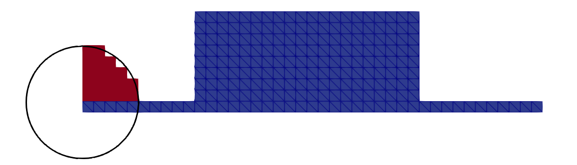
Subsequently, as shown in Fig. 2.17a, a circle is drawn, centred at the interface between a filled voxel and its empty neighbouring voxel. This circle represents the so-called advection kernel or advection distribution, which encompasses all the geometric information of the emulated process. A circle corresponds to uniform surface movement in all directions and is thus used to emulate a perfectly isotropic deposition processes.
After the advection kernel has been placed at the interface, all empty cells within the kernel are set to filled, as indicated in Fig. 2.17a. Depending on the exact shape of the advection kernel, different processes can be emulated. Repeating this procedure for all points on the surface leads to the formation of a new material which is a geometrically accurate representation of an isotropically deposited film on top of the initial material.
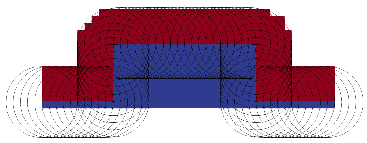
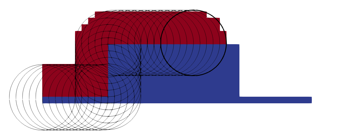
(c) Once all circles have been drawn, their union and thus the resulting geometry accurately represents the result of a perfectly isotropic deposition process.
Figure 2.17: Advection of a voxel-based explicit mesh for the emulation of an isotropic deposition process. The centre of each advection kernel is found by taking a filled voxel with a neighbouring empty cell and placing the centre of the kernel at their interface. Several deposition kernels (black circles) are used at the interface between the filled initial cells (blue) and empty cells to draw the new surface. All empty cells within a distribution are filled with the new material.
Fig. 2.17 shows this procedure after the first kernel was drawn, at some point in time during the advection and the final result showing the entire new material. Some of the problems of the geometric advection method are also visible in this figure. Due to the limited resolution of the voxel-based material representation, sub-grid distances cannot be represented accurately [78]. This leads to the small gap between the advection kernels and the new material on the top surface and to stepped corners which should be smooth and round. The metric used to determine whether a voxel is inside or outside of the advection kernel also has a great impact on the final result. If the centre point is used, more than half of the volume of the voxel might actually be filled with the new material, but the voxel is left empty because the centre is not inside the new material. Additionally, the top surface in Fig. 2.17c is not advected as far as the advection kernels reach and thus the new surface is not moved far enough. These small inaccuracies can accumulate and ultimately lead to large discrepancies in the final result. Therefore, while the geometric voxel advection offers great computational efficiency and is easily implemented, the limited resolution and possible numerical issues make it unfavourable for many applications [79].
In the example discussed in the previous section, a geometric advection distribution was used to describe the geometric effect the modelled process has on the initial surface. The final surface, after isotropic deposition, was emulated using spherical advection distributions placed on the initial surface. The circle in 2D, or sphere in 3D, implies that the surface is moving at the same speed in all directions. Thereby, the radius of the sphere sets how far the surface has been advanced by the end of the modelled process.
In order to capture the specific geometric behaviour of each process, it must be expressed as a geometric distribution. Given the geometric characteristics of the modelled process, such a distribution must describe how a specific point on the initial surface \(\vec {x}_s\) affects the final interface. In the case of isotropic deposition, it is most natural to express the effect on the final surface in terms of the spherical angles \(\theta _{inc}\) and \(\phi _{az}\)
\( \seteqsection {2} \) \( \seteqnumber {60} \)
\begin{equation} D_{iso}(\vec {x}_s, \theta _{inc}, \phi _{az}) = R_{iso} \quad , \end{equation}
where \(R_{iso}\) is the deposition distance. Since this advection distribution is independent of \(\vec {x}_s\) and the spherical angles, it is isotropic and thus has the same effect everywhere on the initial surface. If the growth distance of a deposition process does depend on some locally varying surface property \(F(\vec {x}_s)\), but is isotropic nonetheless, the radius of the spherical deposition will simply be scaled by this property using
\( \seteqsection {2} \) \( \seteqnumber {61} \)
\begin{equation} D_{iso}(\vec {x}_s) =F(\vec {x}_s) R_{iso} \quad . \end{equation}
If the process is not isotropic and therefore has some directionality, the geometric distribution must have a non-spherical shape. There are no general limitations on the shape or complexity of the spherical distribution, other than it being single valued in all \(\vec {x}_s, \theta _{inc}, \phi _{az}\). This must be the case as it represents the distance by which the surface at \(\vec {x}_s\) would move under the modelled process to form the final interface, if there were no other initial surface points. As the surface can only be moved by a single distance in each direction, the geometric advection distribution must be single-valued.
For certain distributions it may be more natural to express them in terms of other coordinate systems in which it is easier to represent the shape of the distribution. For example, perfectly directional processes which only move the surface in one spatial direction and not in any other are more naturally expressed using Cartesian coordinates. However, no matter what coordinate system is used to represent the geometric distribution, it must be single valued for all combinations of its arguments.
Signed Distance Calculation Using Geometric Distributions
By considering this definition of geometric advection distributions, the voxel-based approach presented in the previous section (see Fig. 2.17) can be extended to the LS method [106].
The simplest approach would be to generate the implicit surface of a geometric advection distribution, centre it at each initial surface point and then use Boolean operations to generate the final surface. This would entail iterating
over the initial surface once for every grid point of the final surface, making it computationally inefficient. However, by considering the geometric nature of the SDF used to describe implicit surfaces, it is possible to construct the
final surface directly.
Using the geometric approach, a point on the final surface does not evolve from its neighbouring points but is rather set directly. Therefore, the signed distance \(d_s\) of each active grid point \(\vec {a}\) on the new surface may be calculated independently of all others. To calculate the signed distance value, first a possible new surface point \(\vec {P}_{cand}\) referred to as candidate point is selected, as shown in Fig. 2.18.

Figure 2.18: A geometric distribution (dashed red) describing isotropic growth, used to calculate the signed distance \(d_s\) for a candidate point \(\vec {P}_{cand}\) (blue) from one point of the initial surface \(\vec {P}_{cont}\) (red). The growth distance \(R_{iso}\) is equal for all directions of the distance vector \(\vec {v}\). The set of all initial points are shown in black and the set of all candidate points in orange.
Next, the signed distance value of this point is calculated using each initial surface point \(\vec {P}_{cont}\), called contribute point, at a time. First, the geometric distribution is centred at \(\vec {P}_{cont}\), shown in Fig. 2.18 for an isotropic deposition. In order to calculate the signed distance \(d_s\), the distance vector \(\vec {v}\) from \(\vec {P}_{cont}\) to \(\vec {P}_{cand}\) is calculated. The geometric advection distribution is then used to find the advection distance of the process in the direction of \(\vec {v}\). The signed distance of the new surface to the point \(\vec {P}_{cand}\) is then given by
\( \seteqsection {2} \) \( \seteqnumber {62} \)
\begin{equation} d_s(\vec {v}, D(\vec {x}_s, \vec {v})) = |\vec {v}| - D(\vec {x}_s, \vec {v}) \quad . \end{equation}
In the case of isotropic deposition, given in Fig. 2.18, this simplifies to
\( \seteqsection {2} \) \( \seteqnumber {63} \)
\begin{equation} d_s(\vec {v}) = |\vec {v}| - D_{iso} = |\vec {v}| - R_{iso} \quad . \end{equation}
Hence, the signed distance \(d_s\) of the final surface only depends on \(|\vec {v}|\), the distance to the initial surface, but not on direction or location, as one would expect for isotropic growth everywhere on the surface.
Since \(\phi (\vec {x})\) is scaled to the grid spacing, the new LS value at \(\vec {P}_{cand}\) is given by
\( \seteqsection {2} \) \( \seteqnumber {64} \)
\begin{equation} \phi (\vec {P}_{cand}, t_\text {final}) = \frac {|\vec {v}| - D(\vec {x}_s, \vec {v})}{\Delta g} \quad , \end{equation}
which, for the isotropic case, simply becomes
\( \seteqsection {2} \) \( \seteqnumber {65} \)
\begin{equation} \phi (\vec {P}_{cand}, t_\text {final}) = \frac {|\vec {v}| - R_{iso}}{\Delta g} \quad . \label {eq::sphericalDistribution} \end{equation}
Once this calculation has been performed with all possible active points \(\vec {a}\) of the new surface by setting them as \(\vec {P}_{cand}\), the new LS values \(\phi (\vec {a}, t_\text {final})\) represent a correctly initialised LS describing the final surface. The way in which all the possible combinations of contribute and candidate points are merged to form the final level set will be discussed in the following.
The purpose of the geometric advection algorithm is to identify all necessary candidate points of the new surface and use the geometric advection distributions to find the correct LS value for each of these candidate points. Given the set of possible LS values \(\phi (\vec {P}_{cand}, \{\vec {P}_{cont}\})\) for each candidate point, the algorithm must identify the correct final value for \(\phi (\vec {P}_{cand})\). In the following, the algorithm will be presented using the isotropic deposition example of the previous section for simplicity. Differences in the algorithm for general geometric advection distributions will be discussed thereafter.
Condition for Choosing the Final LS Value
Isotropic deposition corresponds to a positive and constant surface velocity function. Therefore, the velocity field \(V(\vec {x}, t) = R\) for \(R\geq 0\) in Eq. (2.30) and the numerical LS equation may be written as
\( \seteqsection {2} \) \( \seteqnumber {66} \)
\begin{equation} \phi (\vec {g}, t_\text {final}) = \phi (\vec {g}, t) - R ||\nabla \phi (\vec {g}, t)||_2 \quad . \end{equation}
By definition, \(||\nabla \phi (\vec {g}, t)||_2 > 0\) and \(R\) must be positive. Therefore, all level set values must decrease when advected under a velocity field describing isotropic deposition. Intuitively, this can be imagined as more and more grid points moving inside the surface and thus becoming negative, while grid points outside of the surface are closer to the surface than before and thus their LS value must be smaller.
As all LS values must decrease, the smallest value of a set of possible level set values for a point \(\vec {P}_{cand}\) correctly describes the final LS since it implies the farthest movement of the surface:
\( \seteqsection {2} \) \( \seteqnumber {67} \)
\begin{equation} \phi (\vec {P}_{cand}, t_\text {final}) = \min \left ( \phi (\vec {P}_{cand}, \{\vec {P}_{cont}\}, t_\text {final}) \right ) \quad . \label {eq::geometricMinimal} \end{equation}
Note that this only holds for a deposition process, since all LS values decrease in size. The opposite is the case for an etching process, where the maximum value must be chosen, since every LS value must increase.
The Algorithm
Using the above definition for choosing the correct LS values, the algorithm in Fig. 2.19 is used to generate the final surface only from the initial LS and a geometric advection
distribution.
The algorithm is described in detail in the following, with the most important steps depicted in detail in Fig. 2.20:
1. Generate Explicit Points: First, points on the initial surface must be generated so geometric advection distributions can be centred on them. The resulting point cloud should represent the surface with enough accuracy to not loose any features. However, since the final LS has a finite resolution, numerous additional points will not provide added benefit, while increasing the number of signed distance calculations and therefore computational effort. The ideal resolution of the initial surface is thus on the order of the grid spacing. As presented in Section 2.3.2.3, the LS can be used to quickly generate points on the surface using the closest point approximation [60]. Since grid points are used to generate these points, they are automatically separated by roughly one grid spacing. Therefore, centring one geometric advection distribution at each point will produce the expected final surface.
2. Identify Candidate Points: Find the grid points, which will likely be active grid points of the new level set and thus may be involved in describing the final surface. These are shown as orange and blue points in Fig. 2.20a and should represent the minimal set of new LS points. Ideally, the set of candidate points \(\{ \vec {P}_{cand} \}\) is exactly equivalent to the set of active points \(\{ \vec {a} \} \) of the final LS . While it is possible to treat all grid points as candidate points, keeping the number of candidate points low is key to an efficient algorithm, as it drastically reduces the number of time-consuming calculations of \(\phi (\vec {P}_{cand}, \vec {P}_{cont})\). An efficient implementation for identifying the minimal set of candidate points is discussed in Section 4.2.7.1.
3. Iterate over Candidate Points:
(a) Identify Contribute Points: For each candidate point, the set of contribute points which might affect the formers final value must be identified. Again, this could include all initial surface points, however this set should also be as small as possible in order to save computation time. Since active points of the new surface must lie on the boundary of the geometric advection distribution, a simple bounding box approach can be used to identify possible contribute points, as shown in Fig. 2.20b. Depending on the exact shape of the geometric advection distribution, there might be more efficient methods to identify contribute points given a specific candidate point. However, the bounding box approach can be used universally and thus provides a robust strategy while being reasonably efficient for most advection distributions encountered in process simulation, such as spheres, boxes, or ellipsoids.
(b) Calculate New Level Set Value: For each of the just-identified contribute points, the LS value which they would produce at the candidate point is calculated. This means that \(\phi (\vec {P}_{cand}, \vec {P}_{cont}, t_\text {final})\) is evaluated as shown in Fig. 2.20c. Using Eq. (2.67), the lowest of these values is chosen as the final LS value \(\phi (\vec {P}_{cand}, t_\text {final})\). This final value is then checked to see whether the current candidate point will be an active point on the final surface. If it is not, meaning \(|\phi (\vec {P}_{cand}, t_{final})| > \Delta g\), the candidate point will be discarded.
4. Finalise Level Set: Once all candidate points have been considered and their LS values have been calculated, they automatically form a valid new surface. The values of the candidates which were discarded are not required and are thus not considered in the final surface, forming an efficient sparse-field LS. However, the final surface still contains LS values larger than \(0.5\), which are not required for sparse-field LSs and could be removed in a final step. Nevertheless, in regions of high curvature it is beneficial to not only include the \(\mathcal {L}_0\), but also the \(\mathcal {L}_1\) layer and thus allow values up to \(1\) in order to achieve a more robust surface description. Since these values are still required for the algorithm and would have to be removed in an additional step which does not provide great benefits, it is recommended that these values are kept in the final result.

(a) Generate closest surface points (black), find set of candidates \(\{\vec {P}_{cand}\}\) (orange) and select one \(\vec {P}_{cand}\) (blue).

(b) Use bounding box (dashed blue) to find points \(\vec {P}_{cont}\) which may contribute (pink) and select one (red).

(c) Calculate \(\phi (\vec {P}_{cand})\) for all \(\vec {P}_{cont}\) and choose the lowest as the final value (blue).

(d) When all \(\phi (\vec {P}_{cand})\) are calculated, a valid new LS has been constructed automatically.
Figure 2.20: Visualisation of how the algorithm generates the LS describing the final surface from a point cloud of the initial surface.
The criterion for choosing the correct \(\phi (\vec {P}_{cand}, t_\text {final})\) from the set \(\phi (\vec {P}_{cand}, \{\vec {P}_{cont}\}, t_\text {final})\) was defined in Eq. (2.67). For a deposition process, the lowest value leads to the expected surface description, since all values in the LS must decrease. Choosing the minimum of the set of values gives the correct result because this value reflects the farthest movement of the surface under the advection, meaning the contribute point which contributes most to the deposition is kept.
However, this is not the case for etching processes, where all LS values must increase and thus the maximum value corresponds to the farthest movement. Therefore, the criterion for choosing the correct final value changes depending on the geometric advection distribution which must be known in advance, so the same criterion can be applied for all candidate points. Whether the geometric advection distribution describes deposition or etching, is denoted by its sign. In this work,the convention of negative values indicating etching is used.
Since the criterion for choosing the correct LS values must be known in advance, the modelled process cannot include simultaneous deposition in one region and etching in another, as is the case in modern plasma processes [110]. However, such a process can still be modelled by splitting it into two different geometric advection steps, one for etching, followed by a second geometric advection for deposition.
In order to use the geometric advection algorithm in microelectronic simulations, it is essential that multiple materials and differing advection distributions based on the current material can be handled appropriately. Using the layer-wrapping approach described in Section 2.3.2.5, the initial surface must include all lower material and thus represents the union of all materials in the simulation domain. Given a point on the initial surface \(\vec {x}_s\) and the distance vector to a candidate point \(\vec {P}_{cand}\), the material for both can be deduced straight-forwardly. Since the geometric advection distributions are a function of both, the distribution may change according to the material of the initial surface as well as of the final surface at \(\vec {P}_{cand}\). If, for example, a part of the initial surface is covered by a masking material, the geometric advection distribution at these points can be set to zero, leading to the same behaviour as if the material had been masked. Equally, if a material should be etched until an etch stop layer is reached, the geometric advection can be set to \(\phi _{\text {etch stop}}\) if \(\vec {P}_{cand}\) is part of this layer, thus leaving the etch stop material intact. Therefore, no special consideration or change in the algorithm is necessary to incorporate multiple materials since all the information is already included in the geometric advection distribution.
Using geometric advection, the movement of the surface is only described by a distance rather than a velocity used for iterative advection. Therefore, velocity functions which vary in time cannot be modelled using the geometric advection approach without more detailed considerations. The most important limitation is that a geometric advection distribution must be single-valued in all its arguments. Thus, in order to represent this surface movement using a geometric advection, the integral of the surface movement over time must be single valued in every spatial direction from the initial surface. If this is not the case, the process can usually still be modelled using geometric advection, but must be split into several sequential steps of geometric advections. How many steps are necessary and how exactly the process should be split up must be considered for every modelled process individually.
Several important manufacturing processes lead to changes deep within materials, instead of just on their surfaces and interfaces. Some diffusion processes, such as ion implantation [111] or thermal annealing [112], might not affect the interface but rather result in a change of properties inside the material, while others might lead to a change of the interface which is controlled by changing densities inside the material, such as oxidation [113]. The doping concentration may also heavily influence etch rates [114], which is why volume-dependent modelling may be important even when only topographical changes should be simulated.
In order to model these processes, a volume representation is necessary to store all the relevant information wherever it is needed. A simple and commonly applied solution is using a triangular [115] or tetrahedral mesh [113], where each triangle or tetrahedron stores all the necessary information. However, this means that the entire volume has to be represented, which is memory intensive. Since diffusive processes act by diffusing through the material from the surface, usually only the volume directly under the surface needs to be represented in order to model the process appropriately.
A cell-based representation, as discussed in Section 2.3.3.2, is compatible with the level set and can be used to store volume data. Therefore, a sparse approach was developed within this work, similar to the sparse-field LS, in which the volume is split into voxels, centred around a grid point, and information is stored only at required grid points. Using this cell-based representation on the same grid as the LS thus leads to an accurate and robust description of volume properties and their evolution in time. If the change in volume property, such as strain or doping, results in a topographical change, a velocity field \(\vec {V}(\vec {g})\) can be generated from the cell-based representation and used to robustly move the LS surface. Converting the final LS-based result to filling fractions, as described in Section 2.3.3.2, allows to obtain the final cell-based volume description. This flexible approach allows any type of volume data to be stored and manipulated by different algorithms depending on the application. Therefore, this design allows for ion implantation, diffusion and mechanical stress to be modelled using the most appropriate algorithm, while still keeping the benefits of a LS surface description and minimizing the need for mesh conversions. Since both material representations only store sparse data, this approach is also highly memory efficient.