[
Home ]
[
Home ]
[
Home ]
Using the continuum approach, the material \(\mathcal {M}\) can simply be described by its bounding surface \(\mathcal {S}\), as discussed in Section 2.2.2. If all physical properties of a material are homogeneous, describing the material interfaces is sufficient to capture all the relevant information without having to include a description of the entire volume.
The most straight-forward means to describe a surface is by defining points in space which are found on this surface and connecting them with surface elements. Such representations are referred to as explicit surfaces, because the location of the surface is given explicitly by the points, or nodes, on the surface. This approach is also referred to as segment-based, as the surface is segmented by the elements connecting the nodes [38]. In two-dimensional (2D) simulations, the surface elements are usually straight lines forming a closed loop surrounding \(\mathcal {M}\). The surface normal of each surface element (i.e., straight line in 2D) is usually chosen to point toward the outside of the material, as shown in Fig. 2.2a. By convention, the normal points to the left side when going from the first node of a line segment \(\vec {x}_0\) to the second \(\vec {x}_1\), so the normal vector is given by:
\( \seteqsection {2} \)
\begin{equation} \vec {n} = \begin {pmatrix} (\vec {x}_0 - \vec {x}_1) \cdot \hat {e}_0 \\ (\vec {x}_1 - \vec {x}_0) \cdot \hat {e}_1 \end {pmatrix} \quad , \end{equation}
where \(\hat {e}_i\) is a unit vector in the ith Cartesian direction. Using this method, the order of the nodes of the line segmentation describes which side of the surfaces \(\mathcal {S}\) corresponds to the inside of the material \(\mathcal {M}\).
In three-dimensional (3D), the simplest surface elements to describe \(\mathcal {S}\) are triangles which must form a closed volume describing \(\mathcal {M}\), as shown in Fig. 2.2. As in the 2D description, the surface normals point outwards from \(\mathcal {M}\) to indicate which side of the surface is inside of the material. The surface normal \(\vec {n}\) is generated by the order of the nodes \(\vec {x}_0, \vec {x}_1, \vec {x}_2\) forming the triangle:
\( \seteqsection {2} \) \( \seteqnumber {2} \)
\begin{equation} \vec {n} = \left ( \vec {x}_1 - \vec {x}_0 \right ) \times \left ( \vec {x}_2 - \vec {x}_0 \right ) \quad . \end{equation}
Since the normal vectors of all elements are known, a point \(\vec {x}\) is inside of \(\mathcal {M}\) if it is inside of every surface element, thus requiring to check all segments to test whether \(\vec {x}\) is inside the material.
Explicit representations are used in many applications, including graphics rendering [39] or computer-aided design (CAD) [40]. Several desirable properties make it a good choice for these applications, such as no limitation on resolution as the position of the surface is given by the location of the surface nodes, which can be placed anywhere in space. Another desirable property is the minimal memory requirement, as surface elements scale with the represented surface area and no extra memory is needed. Additionally, visualisation is straight-forward as all coordinates of the surface elements are known. If a process is dependent on the volume of a material, such as oxidation which is limited by the oxidisable substrate available inside the surface, the volume can be calculated straight-forwardly [41]. Therefore, explicit surfaces are ideal for representing complex shapes at varying resolutions and for extracting geometric properties, such as surface area or volume.
In addition, multiple materials can be represented straight-forwardly, by simply storing several different closed surfaces with a material identifier for each triangle, specifying which material the triangle describes.
Implicit surface representations do not store the location of the surface using nodes defining the exact coordinates, but rather another property is stored, which can be used to find the explicit location of the surface. These values are given by the implicit function \(\phi (\vec {x})\), which returns a value for any point in space \(\vec {x}\). In this work the convention is used that the exact location of the surface is given by the set of \(\vec {x}\) for which \(\phi (\vec {x}) = 0\). Hence, the location of the surface is given implicitly through the function \(\phi (\vec {x})\).
A common choice for \(\phi (\vec {x})\) is the signed distance function (SDF) \(s(\vec {x})\), which returns the shortest distance to the surface \(\mathcal {S}\), defined by surface points \(\vec {x}_s\), from a given point \(\vec {x}\):
\( \seteqsection {2} \) \( \seteqnumber {3} \)
\begin{equation} s(\vec {x}) = \min ||\vec {x}_s - \vec {x}||_2 \quad , \label {eq::sdf} \end{equation}
where \(|| \cdot ||_2\) denotes the Euclidean norm or \(\ell _2\) norm. The SDF is not solved for a variable, but used to find the set of all points \(\vec {x}_c\), which let the SDF go to a specific scalar value \(c\):
\( \seteqsection {2} \) \( \seteqnumber {4} \)
\begin{equation} \{\vec {x}_c\} = \{\vec {x}| s(\vec {x}) = c\} \end{equation}
This set of points is an isocontour of the SDF, i.e. a contour of equal height, which is why this set of level points is referred to as the level set (LS) of \(s\), \(L_c(s)\) [42], giving this method its name. In order to represent a surface, \(c\) is usually chosen to be zero out of convenience [43, 44]. This convention is convenient because the zero LS \(L_0(s)\) describes the exact location of the explicit surface \(\mathcal {S}\):
\( \seteqsection {2} \) \( \seteqnumber {5} \)
\begin{equation} \mathcal {S} = L_0(s) = \left \{ \vec {x}| s(\vec {x}) = 0 \right \} \end{equation}
Hence, the surface is given by all points in space \(\vec {x}\) for which the SDF \(s(\vec {x})\) is zero. Essentially, all points with zero distance to \(\mathcal {S}\) must be on the surface itself, as expected. All points which are not part of \(\mathcal {S}\) store the shortest distance to the surface with their sign denoting whether they are inside or outside of \(\mathcal {M}\). In this work, the convention that points inside of \(\mathcal {M}\) are negative is followed. Hence, if \(\phi (\vec {x}) \leq 0\), the point \(\vec {x}\) must be inside the material or on its surface and outside otherwise. This makes it very simple to check whether a point is part of \(\mathcal {M}\) without any further considerations, which is not the case when using explicit surfaces.
Since it would be complex to represent all possible surfaces analytically, \(\phi (\vec {x})\) is defined on a rectilinear grid with grid spacing \(\Delta g\), storing its value at every grid point \(\vec {g}\). For numerical stability and simplicity, \(\phi (\vec {x})\) is then normalised to the grid spacing, such that the distance between two grid points is unity. In order to initialise \(\phi (\vec {g})\) from an explicit surface, a signed distance transform is used to construct the SDF at all grid points from the points \(\vec {x}_s\) of the explicit surface \(\mathcal {S}\) bounding the volume \(\mathcal {M}\):
\( \seteqsection {2} \) \( \seteqnumber {6} \)
\begin{equation} \label {eq::LS_initialisation} \phi (\vec {x}, \mathcal {M}) = \frac {1}{\Delta g} \left \{ \begin {array}{@{}ll@{}} - s(\vec {g}), & \text {for $\vec {g} \in \mathcal {M}$} \\ 0, & \text {for $\vec {x} \in \mathcal {S}$} \\ + s(\vec {g}), & \text {for $\vec {g} \notin \mathcal {M}$} \end {array}\right . \end{equation}
For simplicity, the dependency of \(\phi (\vec {x})\) on \(\mathcal {M}\) is not written explicitly every time, but was added here for clarity. Thus, after initialisation, all grid points store the normalised signed distance to the original surface, which means that the LS values \(\phi (\vec {x})\) are not equivalent to the SDF defined in Eq. (2.3) anymore due to the additional scaling. However, this scaling does not affect the signed distance property of \(\phi (x)\) and can thus be applied without further consideration.
In the LS method discussed above, all grid points in the simulation domain hold the signed distance to the surface \(\mathcal {S}\). Therefore, the number of grid points used to store the location of \(\mathcal {S}\) scale with volume as opposed to surface area, which would be the ideal case, achieved only using explicit surface representations [45]. In the narrow band method, the number of required grid points \(\vec {g}\) is reduced, by considering that only grid points close to the surface contribute significantly to the surface description [46].
The contribution of a grid point to the surface description depends on its distance to the surface and thus its LS value \(\phi (\vec {g})\). Therefore, it is useful to classify points into layers \(\mathcal {L}_i\), based on their LS value:
\( \seteqsection {2} \) \( \seteqnumber {7} \)
\begin{equation} \label {eq::LS_layers} \mathcal {L}_i = \left \{ \begin {aligned} \{\vec {x} ~ &| & ~ i - \tfrac {1}{2} \leq &\phi (\vec {x}) < i + \tfrac {1}{2} & & \}, & &\text {for $i < 0$} \\ \{\vec {x} ~ &| & ~ - \tfrac {1}{2} \leq &\phi (\vec {x}) \leq \tfrac {1}{2} & & \}, & &\text {for $i = 0$} \\ \{\vec {x} ~ &| & ~ i - \tfrac {1}{2} < &\phi (\vec {x}) \leq i + \tfrac {1}{2} & & \}, & &\text {for $i > 0$} \end {aligned} \right . \end{equation}
Layer \(\mathcal {L}_i\) then contains all points in space within one grid spacing around the set \(L_i\).
In the LS method, all layers \(\mathcal {L}_i\) for \(i \in \mathbb {Z}\) are included in the set of grid points, meaning there is no maximum value for \(\phi (\vec {g})\). In the narrow band method, the set of grid points is substantially smaller by only considering the layers \(\mathcal {L}_i\) for \(-\frac {k}{2} < i < \frac {k}{2}\) [47], where \(k\) is the narrow band width. Therefore, only grid points inside the narrow band, the region with thickness \(k \Delta g\) centred around the zero LS \(L_0\), are stored. These grid points are referred to as defined points and are shown in Fig. 2.4. The narrow band width is chosen depending on the needs of the specific application, where lower values result in better memory efficiency, but may also result in loss of accuracy depending on the application. There is no universally ideal narrow band width. Compared to the LS method, memory and computational requirements are thus reduced from \(O(N^D)\) to \(O(N^{D-1}k)\), where \(N\) is the number of grid points in each direction and \(D\) is the number of dimensions.
When the narrow band width \(k\), introduced in Section 2.3.2.1, is reduced to \(1\), only the layer \(\mathcal {L}_0\) is stored. The grid points within this layer are called active points \(\vec {a}\), analogously to the defined points in the narrow band method, and satisfy:
\( \seteqsection {2} \) \( \seteqnumber {8} \)
\begin{equation} |\phi (\vec {a})| \leq \frac {1}{2} \quad , \end{equation}
which is the same as Eq. (2.7) with \(i = 0\). The value of \(\frac {1}{2}\) means that every active grid point has exactly two neighbouring active grid points, as shown in Fig. 2.5. Since there cannot be fewer active grid points without creating a hole in the surface, the resulting LS is the smallest set of points being able to describe a surface robustly. This set of grid points is called sparse field [48] and leads to the optimal \(O(N^{D-1})\) memory scaling behaviour, which is identical to that achieved by explicit methods.
However, this sparse set of points requires additional attention in order to form a valid and efficient surface description. By definition, the surface is described by \(L_0\) which must be located between two grid points of opposite sign. As \(\phi (\vec {x})\) is normalised to the grid spacing \(\Delta x\), only one of the two oppositely signed points will be active, unless for the rare case of both being exactly \(0.5\). However, it is sometimes necessary to generate the neighbour points of active points, for example to compute geometric properties of the surface, as will be discussed in Section 2.3.2.3. Using Fig. 2.6a as a visual guide, the set of active points (red) is used as a starting point to generate the set of nearest neighbour points (blue). As every point should store the distance to different parts of the surface, calculating the required values is not straight-forward. This problem is expressed in the Eikonal equation
\( \seteqsection {2} \) \( \seteqnumber {9} \)
\begin{equation} |\nabla \phi (\vec {x})| F(\vec {x}) = 0 \quad , \end{equation}
which must be solved for every nearest neighbour grid point. The act of calculating neighbouring \(\phi (\vec {x})\) values is usually referred to as re-distancing, reinitialisation, or normalisation when it is applied after moving full grid or narrow band level sets [49]. Currently available numerical methods to obtain the solution to this problem include the fast marching method [44, 50] and variations thereof [51, 52, 53], the fast sweeping method [54, 55, 56] and the fast iterative method [57]. Although some of these methods have optimal scaling properties of \(O(N)\) for \(N\) neighbours to calculate, they may depend on certain assumptions about \(\phi (\vec {x})\) and all of them still require considerable computational effort as the differential equation needs to be solved at every point.
The problem of generating neighbour points can be simplified greatly by choosing a different norm for the SDF describing \(\phi (\vec {x})\) [58]. By changing the norm in Eq. (2.3), the SDF
\( \seteqsection {2} \) \( \seteqnumber {10} \)
\begin{equation} m(\vec {x}) = \min ||\vec {x}_s - \vec {x}||_1 \label {eq::mdf} \end{equation}
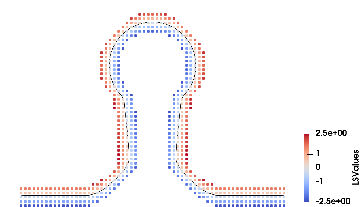
is obtained, where \(|| \cdot ||_1\) represents the Manhattan or \(\ell _1\) norm. The numerical LS function is then defined as in Eq. (2.6) with \(m(\vec {g})\) instead of \(s(\vec {g})\). Every grid point now stores the shortest grid line distance to the interface and \(\phi (\vec {g})\) can be generated by simply checking where \(\mathcal {S}\) intersects the grid lines meeting at \(\vec {g}\). As shown in Fig. 2.6, this norm also leads to a more sparse set of grid points, as the green points in Fig. 2.6a are part of \(\mathcal {L}_0\) using the Euclidean norm, but have higher LS values using the Manhattan norm. Furthermore, neighbour point calculation is straight forward, as a neighbour point can be generated by simply adding unity to an active point. If a neighbouring point has more than one active point, the smallest value plus unity is simply taken as the final LS value, reducing the computational effort to a maximum of \(2 \cdot D\) comparisons and \(1\) addition, a significant reduction in effort when compared to solving a differential equation several times for every neighbour using the \(\ell _2\) norm.
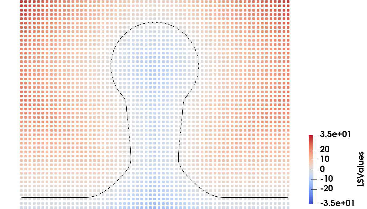
Figure 2.6: Different types of normalisation of the implicit function \(\phi (\vec {x})\). The distance to the surface (black) a) using the Euclidean or \(\ell _2\) norm and b) using the Manhattan or \(\ell _1\) norm. Red points indicate active grid points, blue points indicate values smaller than 1. Green points indicate active grid points which are not necessary for the description of the surface, leading to an inefficient set of grid points.
During simulations, geometric properties of the surface, such as surface normals or curvature are often required [59]. Hence, it is vital to obtain these properties efficiently. When applying the LS method, finding the surface normals and curvature is straight-forward by considering that the explicit surface is the isocontour of the LS at the value \(0\). Since \(\phi (\vec {x})\) increases monotonically with the distance from the explicit surface, the gradient of \(\phi (\vec {x})\) gives the normal direction from the surface. Thus, all geometric properties of the stored surface can be found by calculating derivatives of the LS.
Normal Vectors
One of the most frequently required geometric properties is the normal vector on the surface. Considering that \(\phi (\vec {x})\) is a SDF with the location of the surface being defined as the zero LS \(L_0\), the surface is
simply the isocontour at \(\phi (\vec {x}) = 0\). Since the gradient of a function is always perpendicular to the isocontours of that function, the unit normal vector of \(\phi (\vec {x})\) at the point \(\vec {x}\) is found using
\( \seteqsection {2} \) \( \seteqnumber {11} \)
\begin{equation} \hat {n}(\vec {x}) = \frac {\nabla \phi (\vec {x})}{|| \nabla \phi (\vec {x}) ||_2} \quad . \label {eq::LS_normal} \end{equation}
If \(\vec {x}\) is a point on \(\mathcal {S}\), Eq. (2.11) gives the surface normal at that point.
As the level set is stored numerically on the grid, the gradient is usually computed using finite differences. We therefore define the forward \(D^+_i\) and backward \(D^-_i\) differences as
\( \seteqsection {2} \) \( \seteqnumber {12} \)
\begin{equation} D_i^\pm (\phi (\vec {g})) = \pm \frac {\phi (\vec {g} \pm \Delta g\hat {e}_i) - \phi (\vec {x})}{\Delta g} \quad , \label {eq::forwardDiff} \end{equation}
where \(\hat {e}_i\) is the unit vector in direction \(i\). The numerical derivative, i.e. the gradient \(\nabla \phi (\vec {x})\), on the grid can be approximated by taking the central difference, the average of the forward and backward differences, at the grid point \(\vec {g}\):
\( \seteqsection {2} \) \( \seteqnumber {13} \)
\begin{equation} D_i(\phi (\vec {g})) = \frac {D_i^+(\phi (\vec {g})) + D_i^-(\phi (\vec {g}))}{2} = \frac {\phi (\vec {g}+\Delta g \hat {e}_i) - \phi (\vec {g}-\Delta g \hat {e}_i)}{2 \Delta g} \quad . \label {eq::centralDiff} \end{equation}
Using the definition in Eq. (2.11), the \(i\)th component of the normal vector at the grid point \(\vec {g}\) can thus be approximated using central differences:
\( \seteqsection {2} \) \( \seteqnumber {14} \)
\begin{equation} n_i(\vec {g}) = \frac {1}{|| \nabla \phi (\vec {g})||_2} \frac {\partial \phi (x_i)}{\partial x_i} \approx \frac {D_i(\phi (\vec {g}))}{\sqrt { \sum _{j=1}^{D} D_j(\phi (\vec {g}))^2}} \quad . \end{equation}
The normal vector at the grid point \(\vec {g}\) is a good approximation of the normal at a surface point \(\vec {x}_{cp}\) close to \(\vec {g}\), shown as the green point in Fig. 2.7. Therefore, in order to obtain the surface normals, it is usually sufficient to generate them for every grid point in the layer \(\mathcal {L}_0\), as shown in Fig. 2.8.

Figure 2.7: Normal vector calculation at the grid point \(\vec {g}\) in the LS method using finite differences to approximate the normal at the closest surface point \(\vec {x}_{cp}\) by shifting the grid point a distance \(d\) in the normal direction. This distance is calculated directly from the level set value of \(\vec {g}\) using Eq. (2.15). Blue and red arrows indicate which distances were used to generate the LS values at the neighbouring grid points of \(\vec {g}\).
Closest Point Approximation
If a point on the explicit surface is needed, the closest surface point \(\vec {x}_{cp}\) to a grid point \(\vec {g}\) can be generated directly from the normal and the level set value at \(\vec {g}\) [60]. The point \(\vec
{x}_{cp}\) can be approximated straight-forwardly by shifting the grid point a distance \(d\) along the normal direction \(\hat {n}(\vec {g})\), as indicated by the light blue arrow in Fig. 2.7. Due to the signed distance property of the LS, \(d\) is calculated by simply normalising \(\phi (\vec {g})\) by its gradient:
\( \seteqsection {2} \) \( \seteqnumber {15} \)
\begin{equation} \vec {x}_{cp} (\vec {g}) = \vec {g} - d \hat {n} \approx \vec {g} - \frac {\phi (\vec {g})}{||\nabla \phi (\vec {g})||} \hat {n} \quad \label {eq::close_point} \end{equation}
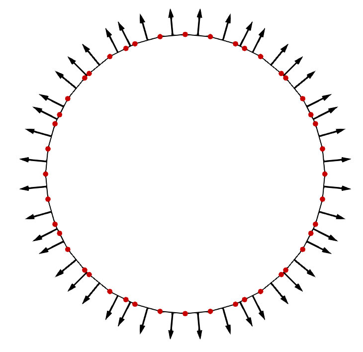
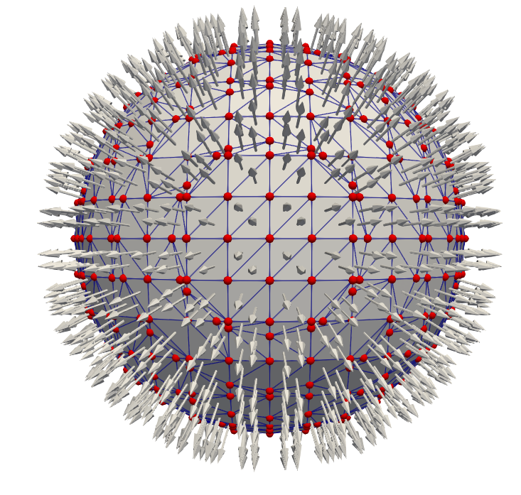
where \(||\cdot ||\) is the norm with which the implicit function was defined. For the SDF defined in Eq. (2.3) this is the \(\ell _2\) norm. If another norm was used, such as the \(\ell _1\) norm for the sparse field LS defined in Eq. (2.10), this norm must be used here to obtain the correct distance to the surface. By repeating this procedure for all grid points within the \(\mathcal {L}_0\) layer, a set of normal vectors spaced roughly by \(\Delta g\) is generated, which is shown for 2D and 3D in Fig. 2.8 analogously to the explicit surfaces in Fig. 2.2.

(a) Shifted active grid points of a circle in 2D.
(b) Shifted active grid points of a sphere in 3D.
Figure 2.8: The closest surface points \(\vec {x}_{cp}\) generated from all grid points in the \(\mathcal {L}_0\) layer shown in the colour of the LS value of the original grid point. The normal vector approximated for each closest surface point is shown as an arrow starting at \(\vec {x}_{cp}\).
Curvature
The curvature of a surface can be used for the detection of features, irregularities or for the smoothing of a surface as will be shown in Section 4.2.5.3. The mean curvature is
given by the second derivative of the implicit function and is expressed as
\( \seteqsection {2} \) \( \seteqnumber {16} \)
\begin{equation} \kappa (\vec {x}) = \nabla \cdot \frac {\nabla \phi (\vec {x})}{||\nabla \phi (\vec {x})||_2} = \nabla \vec {n}(\vec {x}) \quad . \end{equation}
Therefore, the simplest approximation to the mean curvature is the central difference of normals around the current grid point:
\( \seteqsection {2} \) \( \seteqnumber {17} \)
\begin{equation} \kappa (\vec {g}) \approx \sum _{i}^{D} D_i(\vec {n}(\vec {g})) = \sum _{i}^{D} \frac {n_i(\vec {x} + \Delta g \hat {e}_i) - n_i(\vec {x} - \Delta g \hat {e})}{2\Delta g} \end{equation}
Although the above approach gives reasonable results and can be implemented straight-forwardly, a more accurate and robust approximation to the mean curvature in 2D and 3D is given by [44]
\( \seteqsection {2} \) \( \seteqnumber {18} \)
\begin{equation} \kappa (\vec {g}) \approx \frac { \sum _{i \neq j} \left ( D_i^2 D_{jj} - D_i D_j D_{ij} \right ) } { \left ( \sum _{i=1}^{D} D_i^2 \right )^{\frac {3}{2}}} \quad , \end{equation}
where the dependence of the derivatives on \(\phi (\vec {g})\) is not written explicitly and the second order derivatives are given by
\( \seteqsection {2} \) \( \seteqnumber {19} \)
\begin{equation} D_{ij} = D_i(D_j(\phi (\vec {g}))) \quad . \end{equation}
In 3D, the mean curvature is the average of the two principal curvatures. Their product, the Gaussian curvature, can also be calculated directly in the level set [61]:
\( \seteqsection {2} \) \( \seteqnumber {20} \)\begin{align} \kappa _G \approx \frac { \sum _{i \neq j \neq k} \left [ D_i^2 \left ( D_{jj} D_{kk} - D_{jk} \right ) + 2 D_i D_j (D_{ik} D_{kj} - D_{ij} D_{kk}) \right ]} { \left ( \sum _{i=1}^{3} D_i^2 \right )^2} \end{align}
Boolean operations are frequently used to combine two geometric objects in order to generate a new one. In process technology computer aided design (TCAD) this is useful for generating initial geometries or to add masks on top of materials. Boolean operations are defined using the subspaces or materials \(\mathcal {M}_A\) and \(\mathcal {M}_B\) which are combined to result in \(\mathcal {M}_C\). There are three basic Boolean operations which can be used to construct all possible combinations of materials. Using inside or outside of the material as a binary state, these are equivalent to common logic operations:
\( \seteqsection {2} \) \( \seteqnumber {21} \)\begin{align} \text {Union}&: & \mathcal {M}_C &= \mathcal {M}_A \cup \mathcal {M}_B & \text {OR}&: & \mathcal {M}_C &= \mathcal {M}_A \lor \mathcal {M}_B \label {eq::BooleanOR} \\ \text {Instersection} &: & \mathcal {M}_C &= \mathcal {M}_A \cap \mathcal {M}_B & \text {AND}&: & \mathcal {M}_C &= \mathcal {M}_A \land \mathcal {M}_B \label {eq::BooleanAND} \\ \text {Complement} &: & \mathcal {M}_C &= \mathbb {R}^D \setminus \mathcal {M}_A & \text {NOT}&: & \mathcal {M}_C &= \lnot \mathcal {M}_A \label {eq::BooleanNOT} \end{align}
Using surface representations, Boolean operations are used to combine two surfaces and compute the resulting interface. In order to combine explicit surfaces in such a way, the elements making up the surface must be cut and recomputed, requiring expensive intersection and reconstruction algorithms [62]. However, when representing these surfaces as level sets, Boolean operations become simple algebraic expressions which can be can be solved efficiently [63, 64]. In certain applications it was shown to be more efficient to convert to an implicit representation, conduct Boolean operations and then convert back to explicit surfaces instead of performing Boolean operations directly on the explicit surface[65, 66]. The operations on the level sets \(\phi (\vec {x})_A\), \(\phi (\vec {x})_B\) and \(\phi (\vec {x})_C\) corresponding to the Boolean operations in Equations (2.21) to (2.23), respectively, are:
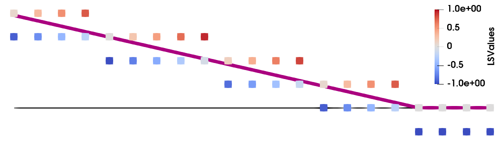
\( \seteqsection {2} \) \( \seteqnumber {24} \)\begin{align} \text {Union}&: & \phi _C(\vec {x}) &= \min (\phi _A(\vec {x}), \phi (_B\vec {x})) \label {eq::LS_OR} \\ \text {Instersection} &: & \phi _C(\vec {x}) &= \max (\phi _A(\vec {x}), \phi _B(\vec {x})) \label {eq::LS_AND} \\ \text {Complement} &: & \phi _C(\vec {x}) &= - \phi _B(\vec {x}) \label {eq::LS_NOT} \end{align} The exact operations to carry out on the level set depends on the convention of the sign denoting inside or outside. Here, the convention of negative values being inside the material are used. Using these expressions, the resulting value \(\phi _C(\vec {x})\) can be computed by simply considering the level set value at the same location \(\vec {x}\) in the level sets \(\phi _A(\vec {x})\) and \(\phi _B(\vec {x})\), as shown in Fig. 2.9. Therefore, a single pass over the grid is sufficient to compute the resulting level set surface, meaning this operation is highly efficient. The efficiency of this approach is especially clear for the complement, where the level set values only have to be inverted.
The simulation of semiconductor fabrication processes requires different types of materials to be represented accurately. The process flow in Section 1.1 requires more than 10 different materials to be represented inside one simulation domain. As discussed in Section 2.3.1, several different materials can be stored straight-forwardly using explicit meshes. However, using the LS method, only one single surface can be represented, as the LS only stores the signed distance to the boundary. Hence it is necessary to store one level set for each material. Storing the level set values on the same grid thus results in a sufficient description of multiple materials within a single simulation domain. However, when thin layers must be represented, the limited resolution of the LS grid leads to numerical difficulties, as shown in Fig. 2.10.
Materials spanning at least two grid points can be represented accurately. However, if there is only one grid point describing both surfaces, the level set values lose their normalisation and at least one of the two boundaries cannot be represented accurately anymore. Fig. 2.10b highlights this symmetric shrinking of the explicit surface if the material is too thin to be represented robustly in a LS. Since the exact location of the surface depends on two neighbouring LS values with opposite sign and the centre grid point can only store one value, both explicit surfaces must be generated using this value, leading to the observed discrepancy. This effect is even stronger if there is no grid point inside the surface since there are no oppositely signed neighbour grid points anymore which could be used to reconstruct the explicit surface. Thus, a thin material layer would disappear in the LS representation, although it may still be almost a grid spacing wide. For physical process simulations, this can lead to large problems, as several fabrication steps, such as plasma etching [67], depend on very thin passivation layers protecting the surface. Furthermore, the deposition of few-atom thick layers [68] is an important fabrication step for various modern devices and therefore must be represented appropriately.

(a) Initial layer, only two grid spacings wide, whose top surface is moved downwards (e.g., etching).

(b) As the layer is thinned to only one grid spacing, the level set values are not normalised anymore, resulting in symmetric shrinking.

(c) Once the last row of grid points is outside of the layer, it ceases to exist, although it should still be almost one grid spacing wide.
Figure 2.10: Different position of a plane surface represented in a level set. The difference to the next position is indicated by red arrows. Grey points indicate the grid, black lines the surface and dashed green lines the correct position of the surface. The level set values of each row are shown to its right.
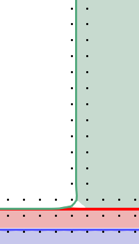
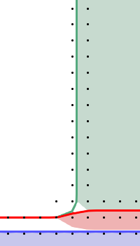
In order to solve this problem, it helps to consider that such thin layers are only formed on thicker substrates and usually do not occur as thin pillars or spikes on their own, but rather as envelopes covering an underlying substrate. Thereby, the bottom surface does not need to be represented at all since the combined knowledge of the top surface and the surface where another material starts are sufficient to describe a thin layer. This essentially describes this material wrapping or enveloping the material below it. The level set which represents the thin layer then describes not only the thin layer material, but also the material on top of which it was grown. The difference is shown in Fig. 2.11 for a thin passivation layer on the surface of a substrate, as commonly encountered in plasma etching processes.
(a) Thin material without layer wrapping.
(b) Layer wrapping used to accurately represent a thin material.
Figure 2.11: a) Thin layers (green) of a material cannot be represented accurately by the level set method. b) If the thin layer is defined on top of another material, as is the case in semiconductor fabrication processes, layer wrapping can be employed to achieve an accurate surface representation (purple) matching the explicit surfaces. The explicit material interfaces are indicated by thin black lines.
The so-called layer wrapping approach thus leads to the expected results and can be used to appropriately describe thin layers. In order to achieve a robust material representation, including thin layers, each LS \(\phi _i(\vec {x})\) must be defined to encompass the union \(\mathcal {M}_i\) of all underlying materials \(\mathcal {M}_j\):
\( \seteqsection {2} \) \( \seteqnumber {27} \)
\begin{equation} \phi _i(\vec {x}) = \phi _i(\vec {x}, \mathcal {M}_i) \quad \mathcal {M}_i = \bigcup _{j=1}^i \mathcal {M}_j \end{equation}
Unwanted effects, such as spaces between materials, symmetric shrinking and disappearance of thin layers are thereby solved robustly, as shown in Fig. 2.12
Great care must be taken when choosing the ordering of materials in order to decide which LS should include and wrap which other surfaces. The most natural and straight-forward ordering is to number the materials by the time of creation during the simulation. The initial substrate is then labelled as material 1, the next one as material 2, and so on. Since a new material can only grow on top of already existing materials and the new layer will wrap those, unwanted side effects such as spaces between materials will be avoided using this strategy.
However, if several materials are introduced at the same time, or complex shapes are simulated with intertwined materials, special considerations may be necessary. Nonetheless, the layer ordering described above leads to robust and predictable behaviour and has been found to be the most straight-forward and efficient means to include thin material films with sub-grid accuracy.
(a) Initial geometry already showing voids if layers are not wrapped.

(b) The thin layer shrinks symmetrically when etched from the top creating a void above the substrate.
(c) Thin layer disappearing completely, leading to a jump of one grid spacing in the process.
Figure 2.12: Level set layers representing different materials during an etch process of a thin layer (red) above a substrate (blue) both protected by a mask (green). The filled areas show the material if no layer wrapping is applied and the coloured lines show the corresponding LS when employing the layer wrapping approach. Voids in the corners of geometries (a), symmetric shrinking (b) and loss of sub grid materials (c) are all handled appropriately using this approach.
Modelling only the surface of a material is sufficient when the physical properties are homogeneous throughout the entire material, as discussed in Section 2.3. However, microelectronic devices are very much dependent on certain properties varying throughout a single material, such as doping concentration [69] or strain [70]. In this case, the entire volume must be represented numerically.
Volumes can be represented numerically using explicit representations, such as a tetrahedral mesh [71]. A volume mesh can also be made up of many other geometric shapes such as cubes or hexahedrons [72]. However, tetrahedrons are usually used as a they can be built from a triangle by simply adding a single node, leading to minimal memory consumption. Such explicit volume meshes are used extensively in the fields of visualisation [73], mechanical engineering [74] and in microelectronic device simulations [75] mentioned in Chapter 1. Much like explicit surface representations, this approach offers optimum memory efficiency and simple generation of geometric properties. However, certain applications require specific conditions to be met regarding the exact structure of the mesh, such as fulfilling the Delaunay criterion [76]. Furthermore, all parts of the volume must be stored explicitly, so large areas with the same physical properties require more memory than necessary. Additionally, since all tetrahedrons are independent, neighbour information has to be stored separately, leading to additional overhead [77].
Another technique for storing volume information numerically is achieved when the simulation space is split into a rectilinear grid, similar to the grid used in the LS method. Therefore, the simulation space is now divided into squares in 2D and cubes in 3D. The simulation space in this method is thus split into cells of equal size, which is why it is usually referred to as a cell-based volume [78]. Each cell is then assigned a number denoting the material the cell represents and a filling fraction \(\mathit {ff}\), denoting how much of the cell is filled with the respective material. The filling fraction is usually bound to the range \([0, 1]\) so that the sum of all filling fractions in a cell always equals unity.
Explicit Volumes
In the simplest case, the filling fraction is binary, meaning the cell is either entirely occupied by the material or empty. This way, there is no need to store a filling fraction. Storing only a material identifier specifying which material
the cell belongs to is sufficient. Therefore, the material is described by a collection of squares or cubes, which form an explicit volume description, as mentioned above. This method is referred to as voxel-based volume
representation [79] and leads to stepped interfaces between materials since the resolution is limited by the size of the voxels. Therefore, high resolutions are required in order to achieve satisfactory final geometries with precise
contours. If the size of individual voxels is close to the size of physical atoms, this approach can be considered for the application in atomistic modelling which enables the simulation of surface reactions in great detail, as well as
atomistic effects such as diffusion or ion implantation [80].
Implicit Volumes
If the filling fraction is a real number, this method is very similar to the LS method, since it represents the material boundary implicitly on a grid. Therefore, this type of cell-based representation is called cell set (CS) and a simple
surface is shown in Fig. 2.13. Due to the strong similarities in the fundamental concepts, cell-based methods share the same shortcomings as level sets, such as lacking memory efficiency,
although this can be solved employing techniques analogous to the sparse field method.

(a) Cell-based representation of a curved boundary of a material. The numbers in the cells represent the filling fraction stored in the respective cell.

(b) Sparse field LS for the same curved boundary from (a), storing the signed distances to the interface.
Figure 2.13: Comparison of a cell-based material and a sparse field LS. While the former is intrinsically associated with volume, level set representations describe an interface or boundary. However, both share common properties as they both represent a material boundary implicitly.
Algorithms associated with describing changing materials using cell-based methods are not as efficient as those developed for the LS method [81]. Although the filling fractions can be used for the calculation of explicit material interfaces [82], they often require complex algorithms to generate the explicit surface from filling fractions alone [83]. Since the exact position of a material inside a cell is not known, the explicit surface needs to be approximated using several neighbouring cells. Furthermore, the precise calculation of the surface normal requires a large number of neighbouring cells as there is no signed distance property as in the LS which could be used. It is therefore not possible to robustly determine the exact location of the surface, especially if there are several different materials present inside one cell. Therefore, the level set method is more appropriate for representing material boundaries.
Due to their similarities, both implicit cells and LSs can be defined on the same grid, where the level set is used to store the exact location of the surface, while the cell-based volume representation is used to store volumetric data, such as doping concentration, strain, or the number of impurities. When the two representations are combined, it is sometimes necessary to convert between them. For example, the surface is advanced in the LS, resulting in the need to also update the filling fraction values. Considering the geometric nature of both functions, namely the distance from the surface for the LS and the volume of the cell inside the boundary for the CS, their underlying implicit functions are closely related. For the conversion to the cell-based representation, the explicit surface can be found using the level set values and the volume inside the cell at the interface is calculated as shown in Appendix A. In one-dimensional (1D) space, the filling fraction \(\mathit {ff}(\vec {x})\) and the LS are related by
\( \seteqsection {2} \) \( \seteqnumber {28} \)
\begin{equation} \mathit {ff}(\vec {x}) = \left \{ \begin {aligned} &0, & &\text {for } & 0.5 < &\phi (\vec {x}) \\ &0.5 - \phi (\vec {x}), & &\text {for } & -0.5 \leq &\phi (\vec {x}) \leq 0.5 \\ &1, & &\text {for } & &\phi (\vec {x}) < -0.5 \\ \end {aligned} \right . \label {eq::LS_vs_FF1D} \end{equation}
This simple relationship is shown in Fig. 2.14a. Note that the axis for the filling fraction is inverted and that, in the interval \([-0.5, 0.5]\), the LS value and the filling fraction only differ by a constant offset of \(0.5\). Outside of this interval, the two functions differ since the filling fraction cannot be less than \(0\) or more than \(1\).
In higher dimensions, the filling fraction is also dependent on the normal vector of the surface, as shown in Fig. 2.14b. The exact relationship is described in Appendix A, where the simple relationship in Eq. (2.28) is only valid if the normal vector is parallel to a grid axis. However, for non-zero angles to the grid \(\gamma \), the function relating the filling fraction and the level set becomes smoother, as highlighted by the inset in Fig. 2.14b. The maximum difference occurs at an angle of \(\gamma = \pi /4\), where the filling fraction differs by \(~0.04\) in 2D. The 1D solution in Eq. (2.28) is therefore a simple approximation for any 2D case, but may lead to an error of up to \(4\%\). Although this approximation might be sufficient for some applications, the error is too large to tolerate for sophisticated physical simulations. Since the surface normal of a level set can be generated straight-forwardly, as described in Section 2.3.2.3, there is no need to use this simple approximation and the accurate CS values can be calculated instead.
The inverse problem, converting a CS to a LS, is not always possible unambiguously. In 1D, a sparse field LS can be generated by simply inverting Eq. (2.28). However, the relationship between the filling fraction and the LS value is more complex in higher dimensions and depends on the surface normal, as shown in Fig. 2.14b. Since the filling fraction does not store information about the location of the surface, it is not possible to calculate the surface normal from the filling fractions alone. This can be visualised by considering that \(\mathit {ff}(\vec {x})\) is not a straight line in Fig. 2.14b, meaning that it does not represent a signed distance. Therefore, a robust conversion from a CS to a LS is not possible in dimensions higher than \(1\).
Figure 2.14: Relationship between the level set values and filling fractions for a) 1D and b) 2D representations. In 1D, the filling fraction (red) follows a straight line (dotted red) in the allowed interval \([0, 1]\), which is given by Eq. (2.28). In dimensions higher than \(1\), the relationship is dependent on the normal vector, where \(\gamma \) is the angle between the normal vector and a grid axis. In the interval \(\gamma = [0, \pi /2]\) the function is symmetric around \(\gamma =\pi /4\) and then repeats periodically.