Emulation and Simulation of
\(\newcommand \ensuremath [1]{#1}\)
\(\newcommand \footnote [2][]{\text {( Footnote #1 )}}\)
\(\newcommand \footnotemark [1][]{\text {( Footnote #1 )}}\)
\(\newcommand {\LWRframebox }[2][]{\fbox {#2}} \newcommand {\framebox }[1][]{\LWRframebox } \)
\(\newcommand {\setlength }[2]{}\)
\(\newcommand {\addtolength }[2]{}\)
\(\newcommand {\setcounter }[2]{}\)
\(\newcommand {\addtocounter }[2]{}\)
\(\newcommand {\cline }[1]{}\)
\(\newcommand {\directlua }[1]{\text {(directlua)}}\)
\(\newcommand {\luatexdirectlua }[1]{\text {(directlua)}}\)
\(\newcommand {\intertext }[1]{\\ \text {#1}\notag \\}\)
\(\newcommand {\mathllap }[2][]{{#1#2}}\)
\(\newcommand {\mathrlap }[2][]{{#1#2}}\)
\(\newcommand {\mathclap }[2][]{{#1#2}}\)
\(\newcommand {\mathmbox }[1]{#1}\)
\(\newcommand {\clap }[1]{#1}\)
\(\newcommand {\LWRmathmakebox }[2][]{#2}\)
\(\newcommand {\mathmakebox }[1][]{\LWRmathmakebox }\)
\(\newcommand {\cramped }[2][]{{#1#2}}\)
\(\newcommand {\crampedllap }[2][]{{#1#2}}\)
\(\newcommand {\crampedrlap }[2][]{{#1#2}}\)
\(\newcommand {\crampedclap }[2][]{{#1#2}}\)
\(\newenvironment {crampedsubarray}[1]{}{}\)
\(\newcommand {\crampedsubstack }{}\)
\(\newcommand {\smashoperator }[2][]{#2}\)
\(\newcommand {\SwapAboveDisplaySkip }{}\)
\(\require {extpfeil}\)
\(\Newextarrow \xleftrightarrow {10,10}{0x2194}\)
\(\Newextarrow \xLeftarrow {10,10}{0x21d0}\)
\(\Newextarrow \xhookleftarrow {10,10}{0x21a9}\)
\(\Newextarrow \xmapsto {10,10}{0x21a6}\)
\(\Newextarrow \xRightarrow {10,10}{0x21d2}\)
\(\Newextarrow \xLeftrightarrow {10,10}{0x21d4}\)
\(\Newextarrow \xhookrightarrow {10,10}{0x21aa}\)
\(\Newextarrow \xrightharpoondown {10,10}{0x21c1}\)
\(\Newextarrow \xleftharpoondown {10,10}{0x21bd}\)
\(\Newextarrow \xrightleftharpoons {10,10}{0x21cc}\)
\(\Newextarrow \xrightharpoonup {10,10}{0x21c0}\)
\(\Newextarrow \xleftharpoonup {10,10}{0x21bc}\)
\(\Newextarrow \xleftrightharpoons {10,10}{0x21cb}\)
\(\newcommand {\LWRdounderbracket }[1]{\underline {#1}}\)
\(\newcommand {\LWRunderbracket }[2][]{\LWRdounderbracket {#2}}\)
\(\newcommand {\underbracket }[1][]{\LWRunderbracket }\)
\(\newcommand {\LWRdooverbracket }[1]{\overline {#1}}\)
\(\newcommand {\LWRoverbracket }[2][]{\LWRdooverbracket {#2}}\)
\(\newcommand {\overbracket }[1][]{\LWRoverbracket }\)
\(\newcommand {\LaTeXunderbrace }[1]{\underbrace {#1}}\)
\(\newcommand {\LaTeXoverbrace }[1]{\overbrace {#1}}\)
\(\newenvironment {matrix*}[1][]{\begin {matrix}}{\end {matrix}}\)
\(\newenvironment {pmatrix*}[1][]{\begin {pmatrix}}{\end {pmatrix}}\)
\(\newenvironment {bmatrix*}[1][]{\begin {bmatrix}}{\end {bmatrix}}\)
\(\newenvironment {Bmatrix*}[1][]{\begin {Bmatrix}}{\end {Bmatrix}}\)
\(\newenvironment {vmatrix*}[1][]{\begin {vmatrix}}{\end {vmatrix}}\)
\(\newenvironment {Vmatrix*}[1][]{\begin {Vmatrix}}{\end {Vmatrix}}\)
\(\newenvironment {smallmatrix*}[1][]{\begin {matrix}}{\end {matrix}}\)
\(\newenvironment {psmallmatrix*}[1][]{\begin {pmatrix}}{\end {pmatrix}}\)
\(\newenvironment {bsmallmatrix*}[1][]{\begin {bmatrix}}{\end {bmatrix}}\)
\(\newenvironment {Bsmallmatrix*}[1][]{\begin {Bmatrix}}{\end {Bmatrix}}\)
\(\newenvironment {vsmallmatrix*}[1][]{\begin {vmatrix}}{\end {vmatrix}}\)
\(\newenvironment {Vsmallmatrix*}[1][]{\begin {Vmatrix}}{\end {Vmatrix}}\)
\(\newenvironment {psmallmatrix}[1][]{\begin {pmatrix}}{\end {pmatrix}}\)
\(\newenvironment {bsmallmatrix}[1][]{\begin {bmatrix}}{\end {bmatrix}}\)
\(\newenvironment {Bsmallmatrix}[1][]{\begin {Bmatrix}}{\end {Bmatrix}}\)
\(\newenvironment {vsmallmatrix}[1][]{\begin {vmatrix}}{\end {vmatrix}}\)
\(\newenvironment {Vsmallmatrix}[1][]{\begin {Vmatrix}}{\end {Vmatrix}}\)
\(\newcommand {\LWRmultlined }[1][]{\begin {multline*}}\)
\(\newenvironment {multlined}[1][]{\LWRmultlined }{\end {multline*}}\)
\(\let \LWRorigshoveleft \shoveleft \)
\(\renewcommand {\shoveleft }[1][]{\LWRorigshoveleft }\)
\(\let \LWRorigshoveright \shoveright \)
\(\renewcommand {\shoveright }[1][]{\LWRorigshoveright }\)
\(\newenvironment {dcases}{\begin {cases}}{\end {cases}}\)
\(\newenvironment {dcases*}{\begin {cases}}{\end {cases}}\)
\(\newenvironment {rcases}{\begin {cases}}{\end {cases}}\)
\(\newenvironment {rcases*}{\begin {cases}}{\end {cases}}\)
\(\newenvironment {drcases}{\begin {cases}}{\end {cases}}\)
\(\newenvironment {drcases*}{\begin {cases}}{\end {cases}}\)
\(\newenvironment {cases*}{\begin {cases}}{\end {cases}}\)
\(\newcommand {\MoveEqLeft }[1][]{}\)
\(\def \LWRAboxed #1!|!{\fbox {\(#1\)}&\fbox {\(#2\)}} \newcommand {\Aboxed }[1]{\LWRAboxed #1&&!|!} \)
\( \newcommand {\ArrowBetweenLines }[1][\Updownarrow ]{#1}\)
\(\newcommand {\shortintertext }[1]{\\ \text {#1}\notag \\}\)
\(\newcommand {\vdotswithin }[1]{\hspace {.5em}\vdots }\)
\(\newcommand {\shortvdotswithin }[1]{ & \hspace {.5em}\vdots \\}\)
\(\newcommand {\MTFlushSpaceAbove }{}\)
\(\newcommand {\MTFlushSpaceBelow }{\\}\)
\(\newcommand \lparen {(}\)
\(\newcommand \rparen {)}\)
\(\newcommand {\vcentcolon }{:}\)
\(\newcommand {\ordinarycolon }{:}\)
\(\newcommand \dblcolon {\vcentcolon \vcentcolon }\)
\(\newcommand \coloneqq {\vcentcolon =}\)
\(\newcommand \Coloneqq {\dblcolon =}\)
\(\newcommand \coloneq {\vcentcolon {-}}\)
\(\newcommand \Coloneq {\dblcolon {-}}\)
\(\newcommand \eqqcolon {=\vcentcolon }\)
\(\newcommand \Eqqcolon {=\dblcolon }\)
\(\newcommand \eqcolon {\mathrel {-}\vcentcolon }\)
\(\newcommand \Eqcolon {\mathrel {-}\dblcolon }\)
\(\newcommand \colonapprox {\vcentcolon \approx }\)
\(\newcommand \Colonapprox {\dblcolon \approx }\)
\(\newcommand \colonsim {\vcentcolon \sim }\)
\(\newcommand \Colonsim {\dblcolon \sim }\)
\(\newcommand {\nuparrow }{\cancel {\uparrow }}\)
\(\newcommand {\ndownarrow }{\cancel {\downarrow }}\)
\(\newcommand {\bigtimes }{{\Large \times }}\)
\(\newcommand {\prescript }[3]{{}^{#1}_{#2}#3}\)
\(\newenvironment {lgathered}{\begin {gathered}}{\end {gathered}}\)
\(\newenvironment {rgathered}{\begin {gathered}}{\end {gathered}}\)
\(\newcommand {\splitfrac }[2]{{}^{#1}_{#2}}\)
\(\let \splitdfrac \splitfrac \)
\( \newcommand {\multicolumn }[3]{#3}\)
\(\newcommand {\ang }[2][]{(\mathrm {#2})\degree }\)
\(\newcommand {\num }[2][]{\mathrm {#2}}\)
\(\newcommand {\si }[2][]{\mathrm {#2}}\)
\(\newcommand {\LWRSI }[2][]{\mathrm {#1\LWRSInumber \,#2}}\)
\(\newcommand {\SI }[2][]{\def \LWRSInumber {#2}\LWRSI }\)
\(\newcommand {\numlist }[2][]{\mathrm {#2}}\)
\(\newcommand {\numrange }[3][]{\mathrm {#2~– #3}}\)
\(\newcommand {\SIlist }[3][]{\mathrm {#2\,#3}}\)
\(\newcommand {\SIrange }[4][]{\mathrm {#2\,#4~– #3\,#4}}\)
\(\newcommand {\tablenum }[2][]{\mathrm {#2}}\)
\(\newcommand {\ampere }{\mathrm {A}}\)
\(\newcommand {\candela }{\mathrm {cd}}\)
\(\newcommand {\kelvin }{\mathrm {K}}\)
\(\newcommand {\kilogram }{\mathrm {kg}}\)
\(\newcommand {\metre }{\mathrm {m}}\)
\(\newcommand {\mole }{\mathrm {mol}}\)
\(\newcommand {\second }{\mathrm {s}}\)
\(\newcommand {\becquerel }{\mathrm {Bq}}\)
\(\newcommand {\degreeCelsius }{\unicode {x2103}}\)
\(\newcommand {\coulomb }{\mathrm {C}}\)
\(\newcommand {\farad }{\mathrm {F}}\)
\(\newcommand {\gray }{\mathrm {Gy}}\)
\(\newcommand {\hertz }{\mathrm {Hz}}\)
\(\newcommand {\henry }{\mathrm {H}}\)
\(\newcommand {\joule }{\mathrm {J}}\)
\(\newcommand {\katal }{\mathrm {kat}}\)
\(\newcommand {\lumen }{\mathrm {lm}}\)
\(\newcommand {\lux }{\mathrm {lx}}\)
\(\newcommand {\newton }{\mathrm {N}}\)
\(\newcommand {\ohm }{\mathrm {\Omega }}\)
\(\newcommand {\pascal }{\mathrm {Pa}}\)
\(\newcommand {\radian }{\mathrm {rad}}\)
\(\newcommand {\siemens }{\mathrm {S}}\)
\(\newcommand {\sievert }{\mathrm {Sv}}\)
\(\newcommand {\steradian }{\mathrm {sr}}\)
\(\newcommand {\tesla }{\mathrm {T}}\)
\(\newcommand {\volt }{\mathrm {V}}\)
\(\newcommand {\watt }{\mathrm {W}}\)
\(\newcommand {\weber }{\mathrm {Wb}}\)
\(\newcommand {\day }{\mathrm {d}}\)
\(\newcommand {\degree }{\mathrm {^\circ }}\)
\(\newcommand {\hectare }{\mathrm {ha}}\)
\(\newcommand {\hour }{\mathrm {h}}\)
\(\newcommand {\litre }{\mathrm {l}}\)
\(\newcommand {\liter }{\mathrm {L}}\)
\(\newcommand {\arcminute }{^\prime }\)
\(\newcommand {\minute }{\mathrm {min}}\)
\(\newcommand {\arcsecond }{^{\prime \prime }}\)
\(\newcommand {\tonne }{\mathrm {t}}\)
\(\newcommand {\astronomicalunit }{au}\)
\(\newcommand {\atomicmassunit }{u}\)
\(\newcommand {\bohr }{\mathit {a}_0}\)
\(\newcommand {\clight }{\mathit {c}_0}\)
\(\newcommand {\dalton }{\mathrm {D}_\mathrm {a}}\)
\(\newcommand {\electronmass }{\mathit {m}_{\mathrm {e}}}\)
\(\newcommand {\electronvolt }{\mathrm {eV}}\)
\(\newcommand {\elementarycharge }{\mathit {e}}\)
\(\newcommand {\hartree }{\mathit {E}_{\mathrm {h}}}\)
\(\newcommand {\planckbar }{\mathit {\unicode {x0127}}}\)
\(\newcommand {\angstrom }{\mathrm {\unicode {x00C5}}}\)
\(\let \LWRorigbar \bar \)
\(\newcommand {\bar }{\mathrm {bar}}\)
\(\newcommand {\barn }{\mathrm {b}}\)
\(\newcommand {\bel }{\mathrm {B}}\)
\(\newcommand {\decibel }{\mathrm {dB}}\)
\(\newcommand {\knot }{\mathrm {kn}}\)
\(\newcommand {\mmHg }{\mathrm {mmHg}}\)
\(\newcommand {\nauticalmile }{\mathrm {M}}\)
\(\newcommand {\neper }{\mathrm {Np}}\)
\(\newcommand {\yocto }{\mathrm {y}}\)
\(\newcommand {\zepto }{\mathrm {z}}\)
\(\newcommand {\atto }{\mathrm {a}}\)
\(\newcommand {\femto }{\mathrm {f}}\)
\(\newcommand {\pico }{\mathrm {p}}\)
\(\newcommand {\nano }{\mathrm {n}}\)
\(\newcommand {\micro }{\mathrm {\unicode {x00B5}}}\)
\(\newcommand {\milli }{\mathrm {m}}\)
\(\newcommand {\centi }{\mathrm {c}}\)
\(\newcommand {\deci }{\mathrm {d}}\)
\(\newcommand {\deca }{\mathrm {da}}\)
\(\newcommand {\hecto }{\mathrm {h}}\)
\(\newcommand {\kilo }{\mathrm {k}}\)
\(\newcommand {\mega }{\mathrm {M}}\)
\(\newcommand {\giga }{\mathrm {G}}\)
\(\newcommand {\tera }{\mathrm {T}}\)
\(\newcommand {\peta }{\mathrm {P}}\)
\(\newcommand {\exa }{\mathrm {E}}\)
\(\newcommand {\zetta }{\mathrm {Z}}\)
\(\newcommand {\yotta }{\mathrm {Y}}\)
\(\newcommand {\percent }{\mathrm {\%}}\)
\(\newcommand {\meter }{\mathrm {m}}\)
\(\newcommand {\metre }{\mathrm {m}}\)
\(\newcommand {\gram }{\mathrm {g}}\)
\(\newcommand {\kg }{\kilo \gram }\)
\(\newcommand {\of }[1]{_{\mathrm {#1}}}\)
\(\newcommand {\squared }{^2}\)
\(\newcommand {\square }[1]{\mathrm {#1}^2}\)
\(\newcommand {\cubed }{^3}\)
\(\newcommand {\cubic }[1]{\mathrm {#1}^3}\)
\(\newcommand {\per }{/}\)
\(\newcommand {\celsius }{\unicode {x2103}}\)
\(\newcommand {\fg }{\femto \gram }\)
\(\newcommand {\pg }{\pico \gram }\)
\(\newcommand {\ng }{\nano \gram }\)
\(\newcommand {\ug }{\micro \gram }\)
\(\newcommand {\mg }{\milli \gram }\)
\(\newcommand {\g }{\gram }\)
\(\newcommand {\kg }{\kilo \gram }\)
\(\newcommand {\amu }{\mathrm {u}}\)
\(\newcommand {\pm }{\pico \metre }\)
\(\newcommand {\nm }{\nano \metre }\)
\(\newcommand {\um }{\micro \metre }\)
\(\newcommand {\mm }{\milli \metre }\)
\(\newcommand {\cm }{\centi \metre }\)
\(\newcommand {\dm }{\deci \metre }\)
\(\newcommand {\m }{\metre }\)
\(\newcommand {\km }{\kilo \metre }\)
\(\newcommand {\as }{\atto \second }\)
\(\newcommand {\fs }{\femto \second }\)
\(\newcommand {\ps }{\pico \second }\)
\(\newcommand {\ns }{\nano \second }\)
\(\newcommand {\us }{\micro \second }\)
\(\newcommand {\ms }{\milli \second }\)
\(\newcommand {\s }{\second }\)
\(\newcommand {\fmol }{\femto \mol }\)
\(\newcommand {\pmol }{\pico \mol }\)
\(\newcommand {\nmol }{\nano \mol }\)
\(\newcommand {\umol }{\micro \mol }\)
\(\newcommand {\mmol }{\milli \mol }\)
\(\newcommand {\mol }{\mol }\)
\(\newcommand {\kmol }{\kilo \mol }\)
\(\newcommand {\pA }{\pico \ampere }\)
\(\newcommand {\nA }{\nano \ampere }\)
\(\newcommand {\uA }{\micro \ampere }\)
\(\newcommand {\mA }{\milli \ampere }\)
\(\newcommand {\A }{\ampere }\)
\(\newcommand {\kA }{\kilo \ampere }\)
\(\newcommand {\ul }{\micro \litre }\)
\(\newcommand {\ml }{\milli \litre }\)
\(\newcommand {\l }{\litre }\)
\(\newcommand {\hl }{\hecto \litre }\)
\(\newcommand {\uL }{\micro \liter }\)
\(\newcommand {\mL }{\milli \liter }\)
\(\newcommand {\L }{\liter }\)
\(\newcommand {\hL }{\hecto \liter }\)
\(\newcommand {\mHz }{\milli \hertz }\)
\(\newcommand {\Hz }{\hertz }\)
\(\newcommand {\kHz }{\kilo \hertz }\)
\(\newcommand {\MHz }{\mega \hertz }\)
\(\newcommand {\GHz }{\giga \hertz }\)
\(\newcommand {\THz }{\tera \hertz }\)
\(\newcommand {\mN }{\milli \newton }\)
\(\newcommand {\N }{\newton }\)
\(\newcommand {\kN }{\kilo \newton }\)
\(\newcommand {\MN }{\mega \newton }\)
\(\newcommand {\Pa }{\pascal }\)
\(\newcommand {\kPa }{\kilo \pascal }\)
\(\newcommand {\MPa }{\mega \pascal }\)
\(\newcommand {\GPa }{\giga \pascal }\)
\(\newcommand {\mohm }{\milli \ohm }\)
\(\newcommand {\kohm }{\kilo \ohm }\)
\(\newcommand {\Mohm }{\mega \ohm }\)
\(\newcommand {\pV }{\pico \volt }\)
\(\newcommand {\nV }{\nano \volt }\)
\(\newcommand {\uV }{\micro \volt }\)
\(\newcommand {\mV }{\milli \volt }\)
\(\newcommand {\V }{\volt }\)
\(\newcommand {\kV }{\kilo \volt }\)
\(\newcommand {\W }{\watt }\)
\(\newcommand {\uW }{\micro \watt }\)
\(\newcommand {\mW }{\milli \watt }\)
\(\newcommand {\kW }{\kilo \watt }\)
\(\newcommand {\MW }{\mega \watt }\)
\(\newcommand {\GW }{\giga \watt }\)
\(\newcommand {\J }{\joule }\)
\(\newcommand {\uJ }{\micro \joule }\)
\(\newcommand {\mJ }{\milli \joule }\)
\(\newcommand {\kJ }{\kilo \joule }\)
\(\newcommand {\eV }{\electronvolt }\)
\(\newcommand {\meV }{\milli \electronvolt }\)
\(\newcommand {\keV }{\kilo \electronvolt }\)
\(\newcommand {\MeV }{\mega \electronvolt }\)
\(\newcommand {\GeV }{\giga \electronvolt }\)
\(\newcommand {\TeV }{\tera \electronvolt }\)
\(\newcommand {\kWh }{\kilo \watt \hour }\)
\(\newcommand {\F }{\farad }\)
\(\newcommand {\fF }{\femto \farad }\)
\(\newcommand {\pF }{\pico \farad }\)
\(\newcommand {\K }{\mathrm {K}}\)
\(\newcommand {\dB }{\mathrm {dB}}\)
\(\newcommand {\kibi }{\mathrm {Ki}}\)
\(\newcommand {\mebi }{\mathrm {Mi}}\)
\(\newcommand {\gibi }{\mathrm {Gi}}\)
\(\newcommand {\tebi }{\mathrm {Ti}}\)
\(\newcommand {\pebi }{\mathrm {Pi}}\)
\(\newcommand {\exbi }{\mathrm {Ei}}\)
\(\newcommand {\zebi }{\mathrm {Zi}}\)
\(\newcommand {\yobi }{\mathrm {Yi}}\)
A Calculating Filling Fractions from Level Set Values
Consider a single cell in a grid. In its centre, there is a point of a level set grid, \(\vec {O} = (0.5, 0.5, 0.5)\). In order to approximate a surface corresponding to this level set point, a plane is constructed using \(\hat {n}\), the
normalised normal vector of the level set at \(\vec {O}\). A point on the plane, \(\vec {P}\) is then found by shifting \(\vec {O}\) in the direction of \(\hat {n}\) by the level set value at \(\Phi (\vec {O})\):
\( \seteqsection {A} \)
\begin{equation} \vec {P} = \vec {O} - \hat {n} \frac {\Phi (\vec {O})}{\mid \nabla \Phi (\vec {O}) \mid } \end{equation}
The plane approximating the surface inside the cell, \(p(\vec {x})\) is therefore defined as
\( \seteqsection {A} \) \( \seteqnumber {2} \)
\begin{equation} \hat {n} \cdot (\vec {x} - \vec {P}) = 0 \end{equation}
Due to the symmetry of the cubic cell, the normal vector can always be mapped into one half/quarter of the first quadrant/octant, bounding the polar angles by \(0 < \theta \le \frac {\pi }{4}\) and \(0 < \phi \le \frac {\pi
}{4}\).
A.1 2D Problem
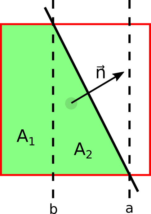
In two dimensions the filling fraction is the area below the line describing the surface within the cell shown in Fig. A.1 . This line is given by
\( \seteqsection {A} \) \( \seteqnumber {3} \)
\begin{equation} p = \frac {\hat {n} \cdot \vec {P}}{n_y} - \frac {n_x}{n_y} x = q - \frac {n_x}{n_y} x \end{equation}
Therefore, the integral is bound to \((0, 0) \le \vec {x} \le (1, 1)\). However, the line might intersect the x-aligned edge of the cell at other points, for \(y = 0\) and \(y = 1\). These intersections, \(a\) and \(b\), are defined by:
\( \seteqsection {A} \) \( \seteqnumber {4} \)
\begin{equation} a = p(y = 0) = \frac {n_y q}{n_x} = \frac {\hat {n} \cdot \vec {P}}{n_x} \quad , \end{equation}
\( \seteqsection {A} \) \( \seteqnumber {5} \)
\begin{equation} b = p(y = 1) = \frac {n_y}{n_x}q - \frac {n_y}{n_x} = \frac {\hat {n} \cdot \vec {P} - n_y}{n_x} \quad , \end{equation}
where both a and b are bound to the interval [0, 1]. The area A is then given by
\( \seteqsection {A} \) \( \seteqnumber {6} \)
\begin{equation} A = \int _{0}^{b} dx + \int _{b}^{a} q - \frac {n_x}{n_y} x dx \end{equation}
Solving this integral gives an expression for the area under curve within the cell, i.e. the filling fraction:
\( \seteqsection {A} \) \( \seteqnumber {7} \)
\begin{equation} A = b + \frac {\hat {n} \cdot \vec {P}}{n_y}(a-b) - \frac {n_x}{2n_y}(a^2 - b^2) \end{equation}

 [
Home ]
[
Home ]