2.3 Oxidation Models
The established macroscopic oxidation model for Si is the Deal-Grove model [62], which provides a relationship between the oxide thickness (X) and the oxidation time (t). The Deal-Grove model has also been applied in a modified form for the oxidation of SiC [63]. However, the oxidation growth cannot be described properly with the Deal-Grove model in the entire thickness region due to the rapid rate decrease in the initial oxidation stage for both Si [64, 65] and SiC [66, 67, 68, 69]. In order to represent the oxidation growth rates below an oxide thickness of a few tens of nanometers, Massoud’s model [64, 65] has been proposed based on empirical observations. Both, in principal, successfully reproduce the growth rate data for SiC oxidation [70, 71, 72]. However, these modeling approaches lacked orientation dependence dictated by the SiC’s crystal structure, which is presented in this work (cf. Section 2.5), in order to enable high accuracy 3D SiC process simulations [73]. Moreover, the exponential term of Massoud’s model is not based on physical considerations, but only on fitting experimental results. To overcome this shortcoming, a Si and C emission model [69] has been proposed based on the interfacial Si and C emission phenomenon [74]. This model introduces Si and C emission into the oxide, which reduce the interfacial reaction rate [75]. However, the growth rate data is restricted to the Si-, C-, and a-face. Therefore, the orientation-dependent oxidation mechanism of SiC cannot be fully validated with experiments. For this reason, the initial oxidation process of SiC has been studied - and is presented in this work (cf. Section 2.7) - based on molecular-level simulations at various temperatures [76] and various SiC faces [77]. All of the oxidation models and molecular level investigations are described in detail in the following sections.
2.3.1 Deal-Grove Model
The basic Deal-Grove oxidation model has been proposed in the 1960s [62]. The model is solely based on two parameters, which are typically extracted from experiments. The model assumes a 1D structure and can be thus reasonably applied only to oxide films grown on planar substrates. The Deal-Grove model assumes that the oxidation process is dominated by the transport and interaction of the oxidant species: 1) The oxidant is transported from the gas ambient to the outer surface of the oxide, 2) the oxidant diffuses through the oxide film, and 3) the oxidant reaches the surface and reacts with Si to form SiO2, i.e., the reaction of the oxidation occurs. The three stages of the oxidation process are illustrated in Figure 2.4. Each of these steps is described as an independent flux F1, F2, and F3. The adsorption of the oxidant species through the surface of the oxide is
\( \seteqsection {2} \) \( \seteqnumber {4} \)
\begin{equation} F_{1} = h \left ( C^{*} - C_{0} \right ), \end{equation}
where h is the gas-phase transport coefficient, C* the concentration of the oxidant in the gas ambient, and C0 the concentration of the oxidant at the SiO2 surface. Assuming saturation of the oxidation in the gas, C* is effectively the solubility limit in the oxide and is related to the partial pressure in the atmosphere by Henry’s law:
\( \seteqsection {2} \) \( \seteqnumber {5} \)
\begin{equation} C^{*} = H \cdot p_\mathrm {x} \end{equation}
px is the partial pressure and H the solute-, solvent-, and temperature-dependent inverse Henry’s law constant. During the oxidation process the diffusivity from the gas to the oxide surface of the oxidant species is much faster than the diffusion through the oxide and the chemical reaction at the surface. Therefore, F1 can be neglected when determining the overall oxidation kinetics.
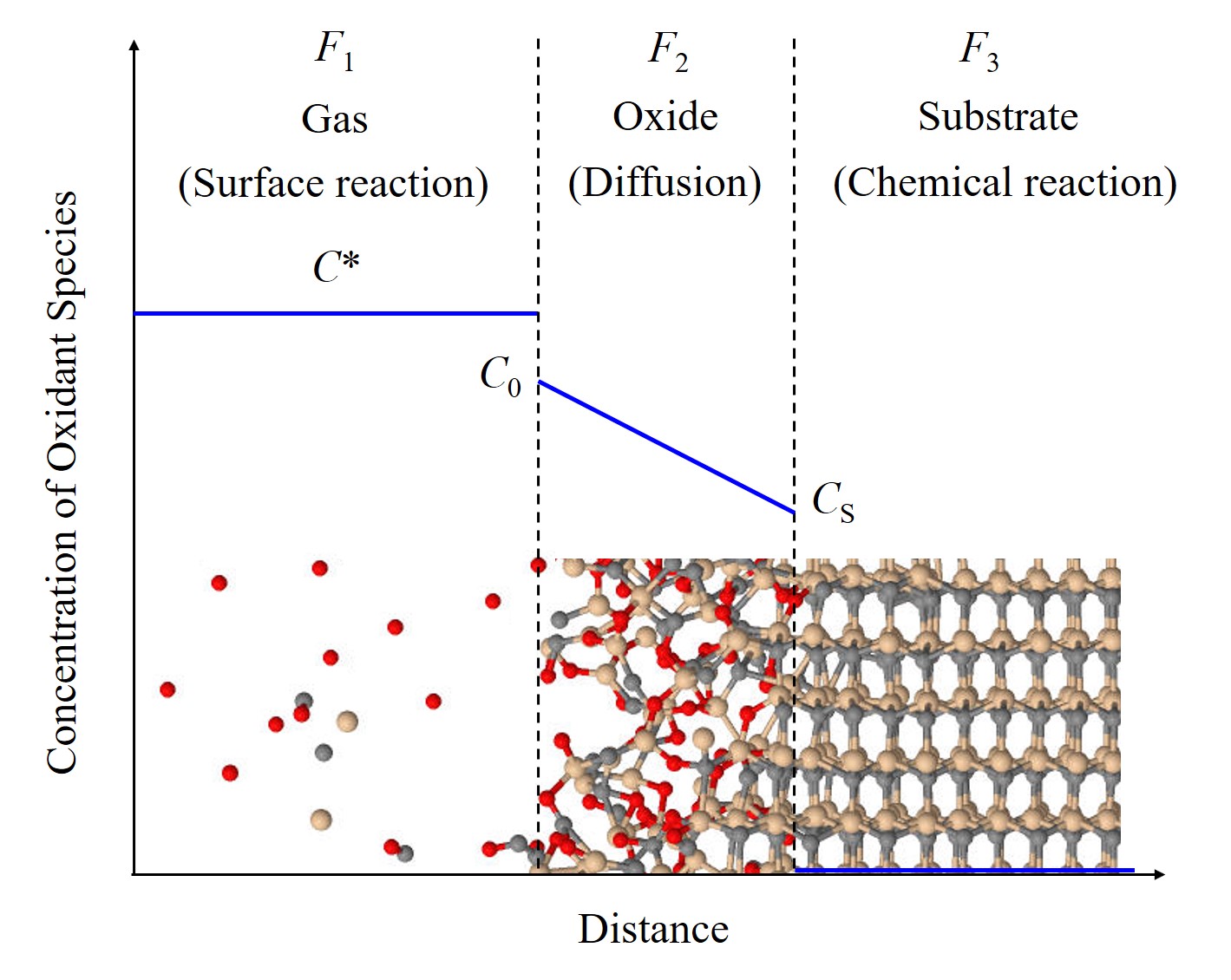
Figure 2.4: Illustration of the oxidation stages described by the Deal-Grove model. F1, F2, and F3 are the three oxidation fluxes and C*, C0, and CS are the concentration of the oxidant in the gas ambient, the concentration of the oxidant at the oxide surface, and the concentration of the oxidant at the interface, respectively. The red, yellow, and gray spheres are O, Si, and C atoms, respectively. The blue lines refer to the concentration of oxidant species as a function of the distance.
The diffusion of the oxidant from the oxide surface to the oxide substrate interface is represented with the flux F2. The diffusion is expressed by Fick’s law:
\( \seteqsection {2} \) \( \seteqnumber {6} \)
\begin{equation} F_{2} = D \frac {\partial C}{\partial x} = D \frac {C_{0}-C_\mathrm {S}}{X} \end{equation}
D the oxidant diffusion coefficient in the oxide, CS the concentration of the oxidant at the interface, and X the thickness of the oxide film. Fick’s law is valid under the assumption of steady state, i.e., when the variables which define the behavior of the system (concentration in this case) are not changing with time. Oxygen molecules do not interact with SiO2 during the diffusion and maintain their molecular form. Thus, the diffusion process is straightforward, i.e., O2 diffuses from the region of high concentration to the region of low concentration. Water vapor molecules, however, interact with SiO2 during the diffusion, thus, the diffusion process is rather complex.
The concentration of the consumed oxidant during the chemical reaction with Si atoms at the substrate surface is described with the flux F3. The chemical oxidation reaction is given by
\( \seteqsection {2} \) \( \seteqnumber {7} \)
\begin{equation} F_{3} = k_\mathrm {s} \cdot C_\mathrm {S} \ , \end{equation}
where ks is the surface rate coefficient. For the sake of simplicity, various reactions at the interface, such as Si-C bond breaking, Si-O bond formation, and O2 or H2O bond dissociation, are here represented by a single reaction coefficient ks. Since steady state conditions are assumed, the three fluxes representing the different stages of the oxidation process must be equal. The rate of the overall oxidation process is determined, i.e., limited, by the rate of the slowest process, such that
\( \seteqsection {2} \) \( \seteqnumber {8} \)
\begin{equation} F_{1} = F_{2} = F_{3} = \frac {C^{*}}{\frac {1}{k_\mathrm {s}} + \frac {1}{h} + \frac {X}{D}} \ . \end{equation}
Since h is very large it can be neglected so that the oxidation reduces to a diffusion of oxidant followed by a chemical reaction. For a thin oxide (ks X/D ≪ 1) the chemical reaction rate is the rate limiting step. On the other hand, for a thick oxide (ks X/D ≫ 1) the rate limiting step is the diffusion.
The oxidation rate is proportional to the flux of the oxidant molecules and is represented by the first order differential equation
\( \seteqsection {2} \) \( \seteqnumber {9} \)
\begin{equation} \frac {dX}{dt} = \frac {F}{N} = \frac {\frac {C^{*}}{N}}{\frac {1}{k_\mathrm {s}} + \frac {1}{h} + \frac {X}{D}} \ , \label {eq:deal-diff} \end{equation}
where N (for dry ≈ 2 · 1022 cm-3 and for wet oxidation ≈ 4 · 1022 cm-3) is the number of oxidant species per unit volume of the grown oxide. The differential equation (2.9) is simplified to
\( \seteqsection {2} \) \( \seteqnumber {10} \)
\begin{equation} \frac {dX}{dt} = \frac {B}{A + 2 X} \ , \end{equation}
where
\( \seteqsection {2} \) \( \seteqnumber {11} \)
\begin{equation} A = 2D \left ( \frac {1}{k_\mathrm {s}} + \frac {1}{h} \right ) \label {eq:parabolic-rate} \end{equation}
and
\( \seteqsection {2} \) \( \seteqnumber {12} \)
\begin{equation} B = 2D \frac {C^{*}}{N} \end{equation}
are the model parameters. B is known as the parabolic rate coefficient and
\( \seteqsection {2} \) \( \seteqnumber {13} \)
\begin{equation} \frac {B}{A} = \frac {C^{*}}{N \left ( \frac {1}{k_\mathrm {s}} + \frac {1}{h} \right )} \label {eq:linear-rate} \end{equation}
is known as the linear rate coefficient of the Deal-Grove model. The linear rate coefficient (2.13) can be simplified under the assumption h ≫ ks to
\( \seteqsection {2} \) \( \seteqnumber {14} \)
\begin{equation} \frac {B}{A} \simeq \frac {C^{*} k_\mathrm {s}}{N} . \end{equation}
The parameters B and B/A are determined experimentally, because not all of the quantities in (2.11) and (2.13) are known. In particular ks is determined by a lot of hidden physical processes associated with the numerous interface reactions. For thin oxides (X < 50 nm) the dominant Deal-Grove parameter is the parabolic rate coefficient (B) and for thick oxides (X > 50 nm) the dominant parameter is the linear rate coefficient (B/A).
In order to obtain an analytical solution of the oxide thickness, the first order differential equation (2.9) is rewritten in the form
\( \seteqsection {2} \) \( \seteqnumber {15} \)
\begin{equation} \left ( A + 2 X \right ) dX = B dt \end{equation}
and integrated over time from 0 to t and over the oxide thickness from Xinit to X, such that
\( \seteqsection {2} \) \( \seteqnumber {16} \)
\begin{equation} \int _{X_\mathrm {init}}^{X} \left ( A + 2 \ X \right ) dX = B \int _{0}^{t} dt . \end{equation}
The solution of the integral yields a quadratic equation:
\( \seteqsection {2} \) \( \seteqnumber {17} \)
\begin{equation} X^2 + A X = B \left ( t + \tau \right ) \end{equation}
τ is the initial oxide thickness-dependent characteristic time of the initial oxidation given by
\( \seteqsection {2} \) \( \seteqnumber {18} \)
\begin{equation} \tau = \frac {X_\mathrm {init}^{2} + A X_\mathrm {init}}{B}. \end{equation}
The oxidation time for a desired oxide thickness can be estimated by
\( \seteqsection {2} \) \( \seteqnumber {19} \)
\begin{equation} t = \frac {X^2 - X_\mathrm {init}^{2}}{B} + \frac {X - X_\mathrm {init}}{B/A}. \end{equation}
The oxide thickness for a desired oxidation time can be estimated by the solution of the quadratic equation
\( \seteqsection {2} \) \( \seteqnumber {20} \)
\begin{equation} X = \frac {A}{2} \left ( \sqrt {1 + \frac {4B}{A^2} \left ( t + \tau \right )} - 1 \right ). \end{equation}
For very long oxidation times, where t ≫ τ and t ≫ A2/4B, the oxide thickness is estimated as
\( \seteqsection {2} \) \( \seteqnumber {21} \)
\begin{equation} X \simeq \sqrt {B \cdot t}. \end{equation}
For very short times, with t ≪ A2/4B, the oxide thickness is estimated as
\( \seteqsection {2} \) \( \seteqnumber {22} \)
\begin{equation} X \simeq \frac {B}{A} \left ( t + \tau \right ). \end{equation}
It is clear by now that the Deal-Grove model yields a simple relationship between the oxide thickness and the oxidation time, which can be determined in a straightforward fashion. In addition, the computational effort for the oxide thickness calculation is, compared to the otherwise necessary solution of the diffusion equation, negligible. Therefore, calculating the oxide thickness is very desirable as it does not significantly increase simulation runtimes. However, as device sizes and geometries began to shrink, the limitations of the Deal-Grove model became evident. It has been observed experimentally that the oxidation growth for the initial stage of oxidation and thin oxide layers is much faster than predicted by the Deal-Grove model [1].
2.3.2 Massoud’s Model
For both Si and SiC the oxidation mechanism for an oxide thickness < 50 nm is extremely fast and non-linear [64, 65, 66, 67, 68, 69]. The causes for the increased oxidation rate are parallel oxidation mechanisms such as Si interstitials injected into the oxide, oxygen vacancies, diffusion of atomic oxygen, surface oxygen exchange, and the effects of a finite non-stoichiometric transition region between amorphous SiO2 and Si. In order to include these oxidation phenomena in the initial stage of the oxidation, the Deal-Grove model has been extended with Massoud’s model [64, 65], which is more accurate, but also a lot more complex.
Massoud’s model is practically the Deal-Grove model with the addition of two exponential terms, which refer to the initial and intermediate oxidation regime [64]. The SiO2 growth rate is thus
\( \seteqsection {2} \) \( \seteqnumber {23} \)
\begin{equation} \frac {dX}{dt} = \frac {B}{A + 2 X} + C_{1} e^{-\frac {X}{L_{1}}} + C_{2} e^{-\frac {X}{L_{2}}}. \end{equation}
B and B/A are the parabolic and the linear rate coefficients, respectively, as defined by the Deal-Grove model, but their values are completely different for Massoud’s model [64]. The two exponential terms represent the rate enhancement in the thin regime. It has been found that the first decaying exponential term C1 e-X/L1 affects the fit only slightly for oxide thicknesses up to ≈ 10 nm [64]. Neglecting this term results in errors of less than 5%, therefore, the empirical expression often includes only the exponential term C2 e-X/L2 in addition to the linear-parabolic term. Massoud’s model is thus commonly expressed as
\( \seteqsection {2} \) \( \seteqnumber {24} \)
\begin{equation} \frac {dX}{dt} = \frac {B}{A + 2 X} + C e^{-\frac {X}{L}}, \label {eq:massoud} \end{equation}
where C is the initial enhancement parameter and L the characteristic length.
Massoud’s model can be expressed as [78]
\( \seteqsection {2} \) \( \seteqnumber {25} \)
\begin{equation} \frac {dX}{dt} = \frac {B + K_{1} e^{-\frac {t}{\tau _{1}}} + K_{2} e^{-\frac {t}{\tau _{2}}}}{A + 2 X}, \label {eq:massoud-2} \end{equation}
in order to obtain an analytical solution. K1 and K2 are the pre-exponential constants and τ1 and τ2 the time constants. Inverting (2.25) gives a convenient expression
\( \seteqsection {2} \) \( \seteqnumber {26} \)
\begin{equation} \left (A + 2 X\right ) dX = \left (B + K_{1} e^{-\frac {t}{\tau _{1}}} + K_{2} e^{-\frac {t}{\tau _{2}}}\right ) dt, \end{equation}
which is then integrated over time from 0 to t and over the oxide thickness from xinit to X, such that
\( \seteqsection {2} \) \( \seteqnumber {27} \)
\begin{equation} \int _{X_\mathrm {init}}^{X} \left ( A + 2 X \right ) dX = \int _{0}^{t} \left (B + K_{1} e^{-\frac {t}{\tau _{1}}} + K_{2} e^{-\frac {t}{\tau _{2}}} \right ) dt. \end{equation}
The solution of the integral yields
\( \seteqsection {2} \) \( \seteqnumber {28} \)
\begin{equation} X^{2} + A \cdot X = B \cdot t + M_{1} \left ( 1 - e^{-\frac {t}{\tau _{1}}} \right ) M_{2} \left ( 1 - e^{-\frac {t}{\tau _{2}}} \right ) + M_{0}, \label {eq:massoud-2-int} \end{equation}
where
\( \seteqsection {2} \) \( \seteqnumber {29} \)
\begin{equation} M_{0} = X_\mathrm {init}^{2} + A \cdot X_\mathrm {init}, \end{equation}
\( \seteqsection {2} \) \( \seteqnumber {30} \)
\begin{equation} M_{1} = K_{1} \cdot \tau _{1}, \end{equation}
and
\( \seteqsection {2} \) \( \seteqnumber {31} \)
\begin{equation} M_{2} = K_{2} \cdot \tau _{2}. \end{equation}
Solving (2.28) yields an analytic expression for the oxide thickness as a function of time:
\( \seteqsection {2} \) \( \seteqnumber {32} \)
\begin{equation} X = -\frac {A}{2} + \sqrt { \left ( \frac {A}{2} \right )^{2} + B \cdot t + M_{1} \left ( 1 - e^{-\frac {t}{\tau _{1}}} \right ) M_{2} \left ( 1 - e^{-\frac {t}{\tau _{2}}} \right ) + M_{0} } \end{equation}
This expression can quite accurately describe the oxidation mechanism of Si and SiC, particularly for very thin oxide layers. However, the exponential term in Massoud’s model is considered non-physical 1, therefore, in order to represent all parameters as physical quantities, another modeling approach is necessary, which is discussed in the following section.
1 A model is considered non-physical when its parameters are empirical, i.e., do not refer to any of the physical quantities, such as, e.g., diffusion coefficients, reaction rates, or solubility limits.
2.3.3 C and Si Emission Model
Among the various Si oxidation models which describe the enhancement in the initial stage of oxidation [74, 79, 80], the interfacial Si emission model shows the best ability to accurately fit the experimental oxidation growth rate data. According to this model, Si atoms are emitted as interstitials into the oxide layer accompanied by oxidation of Si, which is caused by the strain due to the expansion of the Si lattice during the oxidation. The oxidation rate at the interface is initially large and is suppressed by the accumulation of emitted Si atoms near the interface with increasing oxide thickness, i.e., the oxidation rate is not constant, but is a function of the oxide thickness. In the Deal-Grove model and in Massoud’s model, it is considered that the oxide growth occurs only or mainly at the Si-oxide interface. However, according to the interfacial Si emission model [74], oxidation can occur inside the SiO2 layer as well. In addition, for very thin oxide layers some of the emitted Si atoms can diffuse through the oxide layer and reach the oxide surface where diffused Si atoms are then instantly oxidized.
Since the density of Si atoms in 4H-SiC (4.8 · 1022 cm-3 [81]) is almost equal to the density of Si atoms in Si (5.0 · 1022 cm-3 [1]) and the residual carbon is unlikely to exist at the oxide-SiC interface in the early stage of SiC oxidation [82], the stress near or at the interface is considered to be almost identical to the oxidation of Si. Therefore, the atomic emission due to the interfacial stress also accounts for the growth enhancement for the oxidation of SiC. In addition, for the oxidation of SiC, the C emission must be taken into account as well.
The Si and C emission model has been recently proposed for the oxidation of SiC [69], which takes into account both Si and SiC emission into the oxide layer. The emission of Si and C leads to a reduction of the interfacial reaction rate. The reaction equation for SiC oxidation can be written as [82]
\( \seteqsection {2} \) \( \seteqnumber {33} \)
\begin{equation} \begin {split} \mathrm {SiC} + \left ( 2 - \nu _\mathrm {Si} - \nu _\mathrm {C} - \frac {\alpha _\mathrm {CO}}{2} \right ) \mathrm {O}_{2} \rightarrow & \left ( 1 - \nu _\mathrm {Si} \right ) \mathrm {SiO}_{2} + \nu _\mathrm {Si} \mathrm {Si} \\ & + \nu _\mathrm {C} \mathrm {C} + \alpha _\mathrm {CO} \mathrm {CO} + \left ( 1 - \nu _\mathrm {C} - \alpha _\mathrm {CO} \right ) \mathrm {CO}_{2}, \label {eq:SiC-reactions} \end {split} \end{equation}
where αCO is the production ratio of CO and νSi and νC the emission ratio of Si and C, respectively. The interfacial reaction rate k is based on the assumption that the concentration of interstitials does not exceed the solubility limit [69]:
\( \seteqsection {2} \) \( \seteqnumber {34} \)
\begin{equation} k = k_{0} \left ( 1 - \frac {C_\mathrm {Si}^\mathrm {I}}{C_\mathrm {Si}^{0}} \right ) \left ( 1 - \frac {C_\mathrm {C}^\mathrm {I}}{C_\mathrm {C}^{0}} \right ) \end{equation}
k0 is the initial interfacial oxidation rate, CSiI is the concentration of Si interstitials, CCI is the concentration of C interstitials, CSi0 is the solubility limit of Si, and CC0 is the solubility limit of C. This equation implies that the growth rate in the initial stage of oxidation is reduced, because the accumulation rates for Si and C interstitials should be different from each other. Hence, the oxidation time, when the concentration of interstitials saturates, is different between Si and C interstitials.
The diffusion equations are given as [82]
\( \seteqsection {2} \) \( \seteqnumber {35} \)
\begin{equation} \begin {split} \frac {\partial C_\mathrm {Si}}{\partial t} &= \frac {\partial }{\partial x} \left ( D_\mathrm {Si} \frac {\partial C_\mathrm {Si}}{\partial x} \right ) - R_{1} - R_{2} \mathrm {, where } \\ R_{1} &= \eta C_\mathrm {Si}^\mathrm {S} C_ \mathrm {O}^\mathrm {S} \mathrm { and } \\ R_{2} &= \kappa _{1} C_\mathrm {Si} C_\mathrm {O} + \kappa _{2} C_\mathrm {Si} C_\mathrm {O}^{2}, \end {split} \end{equation}
\( \seteqsection {2} \) \( \seteqnumber {36} \)
\begin{equation} \begin {split} \frac {\partial C_\mathrm {C}}{\partial t} &= \frac {\partial }{\partial x} \left ( D_\mathrm {C} \frac {\partial C_\mathrm {C}}{\partial x} \right ) - R_{1}’ - R_{2}’ \mathrm {, where } \\ R_{1}’ &= \eta ’ C_\mathrm {C}^\mathrm {S} C_\mathrm {O}^\mathrm {S} \mathrm { and } \\ R_{2}’ &= \kappa _{1}’ C_\mathrm {C} C_\mathrm {O} + \kappa _{2}’ C_\mathrm {C} C_\mathrm {O}^{2}, \end {split} \end{equation}
and
\( \seteqsection {2} \) \( \seteqnumber {37} \)
\begin{equation} \begin {split} \frac {\partial C_\mathrm {O}}{\partial t} &= \frac {\partial }{\partial x} \left ( D_\mathrm {O} \frac {\partial C_\mathrm {O}}{\partial x} \right ) - R_{1} - R_{1}’ - R_{2} - R_{2}’ - R_{3} \mathrm {, where } \\ R_{3} &= h \left ( C_\mathrm {O}^\mathrm {S} - C_\mathrm {O}^{0} \right ). \end {split} \end{equation}
CSi, CC, and CO are the concentrations of Si, C, and O, respectively. CSiS, CCS, and COS are the concentrations of Si, C, and O at the oxide surface, respectively. DSi, DC, and DO are the diffusion coefficients of Si, C, and O, respectively. η is the oxidation rate of Si interstitials on the oxide surface and η’ the oxidation rate of C interstitials on the oxide surface. κ1 and κ2 are the oxidation rates of Si interstitials on the oxide surface and κ1’ and κ2’ the oxidation rates of C interstitials on the oxide surface. R2 and R2’ represent the absorption of interstitials inside the oxide and are each assumed to consist of two terms [83].
The boundary conditions are determined from the chemical reaction of SiC oxidation (2.33), such that [69]
\( \seteqsection {2} \) \( \seteqnumber {38} \)
\begin{equation} D_\mathrm {Si} \frac {\partial C_\mathrm {Si}}{\partial x} \bigg |_{x=0} = - \nu _\mathrm {Si} k C_\mathrm {O}^\mathrm {I}, \end{equation}
\( \seteqsection {2} \) \( \seteqnumber {39} \)
\begin{equation} D_\mathrm {C} \frac {\partial C_\mathrm {C}}{\partial x} \bigg |_{x=0} = - \nu _\mathrm {C} k C_\mathrm {O}^\mathrm {I}, \end{equation}
and
\( \seteqsection {2} \) \( \seteqnumber {40} \)
\begin{equation} D_\mathrm {O} \frac {\partial C_\mathrm {O}}{\partial x} \bigg |_{x=0} = \left (2 - \nu _\mathrm {Si} - \nu _\mathrm {C} - \frac {\alpha _\mathrm {CO}}{2} \right ) k C_\mathrm {O}^\mathrm {I}. \end{equation}
It should be noted that the oxidation rate in the thick oxide region is limited solely by the in-diffusion of the oxidant [70], and that the out-diffusion of CO in SiO2 is much faster than that of O2 [69]. Thus, it is assumed that the diffusion of CO is independent of the oxidation growth rate.
2.3.4 Summary of Oxidation Models
Each of the described oxidation models has its own advantages and disadvantages, including computational effort and accuracy of predicting the oxide thickness. Taking all the variabilities in account, the most appropriate approach for process TCAD simulations is currently Massoud’s model due to the balance between computational costs and accuracy. The computational effort of Massoud’s model is lower compared to the C and Si emission model, especially when the model is recalculated for many (> 103) crystal directions in 3D simulations. On the other hand, the accuracy of Massoud’s model is higher compared to the Deal-Grove model, in particular for the initial oxide thicknesses. Therefore, Massoud’s model is used as the starting point for the modeling approach throughout the remainder of this work.