In order to find the maximum-likelihood solution for a given Markov chain of some defect (or any other Markov chain), three problems need to be solved:
• Given a HMM  and a sequence of observations
  , the likelihood of the observed sequence
  should be determined. This problem is usually referred to as the forward algorithm, see Section 6.7.1.
• Given a HMM and a sequence of observations , the optimal state sequence  of the underlying Markov model should be found. This problem is usually referred to as the backward algorithm, see Section 6.7.2.
• Given a sequence of observations , the HMM which maximizes the probability should be found. This problem is usually referred to as the parameter update, see Section 6.7.3.
In the literature, the iterative solution to these three distinct problems is often called the Baum-Welch algorithm which can be seen as an EM algorithm for this particular problem [170, 171]. The following description closely follows the excellent tutorials given in [172, 173].
The problem related to the forward algorithm is to determine the likelihood  of observing the sequence given the model .
For a certain sequence of statistically independent inner states, by the definition of  the probability to observe
  given a sequence and a model is given by:
On the other hand, from the definition of  and
and  it follows that the probability of having sequence is
The joint probability to observe and simultaneously is simply the product of (6.41) and (6.42).
To obtain the probability of , one simply has to sum over all possible state sequences:
The problem of this direct approach is its computational expense since a direct calculation would require about  operations. Fortunately, the problem can also be solved more efficiently by using the so-called forward algorithm, which often also is called
  pass. It calculates the probability of a partial observation sequence up to time t, at which the Markov Process is in state
  .
.
The main benefit of this definition is that it can be calculated recursively which reduces the number of operations down to  :
:
1. For all states  calculate
  .
.
2. For all states and times  calculate:
3. From the definition (6.45) it follows that:
Now that the probability to observe a specific sequence of observations for a certain model is known, the hidden part of the HMM should be uncovered. In general, this step is not always necessary as for the classification of data, for example in speech recognition, one could train different models for different words and find the most likely word by performing the forward algorithm on each of the HMMs. How to train models (i.e find the optimal set of parameters) will be discussed in Section 6.7.3. The difference when looking at defects is that usually the information which defect causes a certain set of observations is of minor value. The major interest is to find out the mean transition rates and the sequence of hidden states of a defect with a certain Markov chain as well as its specific threshold voltage shift. For that, the so-called backward algorithm is introduced.
The backward algorithm is designed to find the most likely state sequence given a certain model and a sequence of observations. The forward algorithm defined the probability to observe a sequence up to time  . Now the probability to observe the rest of the sequence (i.e. from
  to
to  ) when being in a specific state at time is sought. The definition is similar to the forward algorithm with the only difference that it starts with the end of the sequence and progresses backwards in time:
Again, the computationally most efficient way is to calculate  recursively as follows:
1. For all states set  .
.
2. For all states and times  calculate:
It should be noted at that point that there are different possible interpretations of ‘most likely’. One is to find the single most likely state sequence for each of the observed sequences, which is done with the Viterbi algorithm [174]. Another
often used criterion is to maximize the expected number of correct states across all sequences. This is not necessarily the same, as the latter criterion could lead to impossible state sequences because it selects the most likely state without taking into regard the probability of the occurrence of the whole state sequence.
However, this optimality criterion should be preferred over the Viterbi algorithm, as it delivers the probabilities of being in each of the states for every instant in time. The matrix holding the probabilities to be in each state for every instant in time with size  is usually referred to as the emission matrix and allows to make soft assignments to states. This means that the exact probabilities are stored for each of the states instead of the Viterbi algorithm, which assigns
  to the most likely state and
  to all others. This is the reason why this method is usually preferred for HMM training.
The probability of being in state at time within the HMM  can be simply expressed in terms of the forward and backward variables as the forward variable defines the relevant probability up to time and the relevant probability after time :
If the values of  are stored, the forward and backward algorithm together deliver an emission matrix sized
  holding the normalized probabilities of being in state . If the actual most likely path is sought, one only needs to take the maximum probability across the states
  for every instant in time.
Up to now, the assumed HMM was fixed. In order to be able to train the model, the last and most important step is to find new estimates for the parameters in order to maximize the probability of the observation sequence.
In general, the parameter update should maximize the probability for an observed sequence given a HMM . In theory this could be done analytically by maximizing (6.44). For practical applications, this approach is, however, infeasible due to the exponentially growing terms in the sum. Instead of using directly, the parameter updates derived in this section maximize Baum’s auxiliary function given in (6.52) (see [171, 172]).
It has been proven that the maximization of  also leads to an increased likelihood
  [171, 172], i.e.
One of the most appealing properties of HMMs is the fact that the parameters can be efficiently re-estimated by the model itself. As the number of states  and the number of observations
  are fixed, only the transition matrix , the emission matrix , and the starting probabilities need to be updated.
For that, one first needs to find the probabilities of being in state at and going to  at . In terms of the model parameters
  ,
,  , and they can be expressed as
where can be calculated from (6.47). On a sidenote, (6.54) is related to (6.50) by
The quantities and  already allow to update all three model parameters by summation over time. For the update of , the sum over the numerator is then the expected number of transitions from to
  whereas the sum over the denominator holds the expected number of transitions away from state (including transitions to state ).
The update of the observation probability matrix to observe the symbol  while being in state is:
Here, the Kronecker delta  is used to mark the states where the HMM is in state and the symbol is observed. The ratio in (6.57) thus is the expected number of times the model is in state with the observation over the expected number of times the model is in state . For the initial probabilities, simply the values of
  are used.
It was proven by Baum and his colleagues, that the HMM with the parameters re-estimated in such a way is either more or equally likely compared to the previous model [175]. The presented algorithm, namely the forward-backward algorithm together with the parameter update is often called Baum-Welch algorithm.
On this occasion, it has to be said that this algorithm is sensitive to local minima in the parameter space. Thus a randomization of the initial parameters is often needed to ensure good training results. Another practical problem are numerical implementation issues, as for example the forward parameters exponentially approach 0 as  increases. To avoid underflow and at the same time maintaining the validity of the formulas for the parameter update, the variables should be transformed in a certain manner as can be found in [173].
In order to train a HMM of a system with multiple defects, two major adjustments to the presented EM algorithm are necessary. One was already mentioned briefly in Section 6.4, namely that the states of the combined transitions matrix of multiple defects are not independent of each other. Since the Baum-Welch algorithm treats all states as independent, direct training would inevitably lead to a drift of the system towards one multi-state defect because of the multiplicative terms from each defect in (6.59).
To mitigate this problem, the algorithm for the parameter update has to be modified. First of all the combined expected transition matrix delivered by (6.56) needs to be split according to the structure of the underlying defects. To
illustrate that we look again at the combined transition matrix of two two-state defects as given in (6.33). For clarity, this time the full combined transition matrix is listed. As the transition matrices of the individual defects have to be row
stochastic, the relations  and
and  hold.
hold.
To find the expected number of transitions of a certain state from a distinct defect, the sum of all transitions involving this particular state in the combined transition matrix has to be calculated. The rows in (6.59) thereby mark the state from which the transition starts, whereas the columns mark the ending state. The usage of masking matrices provides an efficient way to select the states of interest. For that, when constructing the combined matrix, a mask matrix for each state of each defect is calculated. For defect ‘A’ those masks would be:
To find the states in  where for example defect
  has a transition from to , the index-matrix is simply the mask of the starting state times the transposed mask of the ending state. The total number of transitions is obtained by summing over all entries of the selected sub-array.
For the transition rate  , equation (6.61) reads:
It can be seen that the mask matrices  and
and  simply select all the terms of the combined transition matrix, where a transition from state to state
  of defect is observed. The sum over those entries thus is the expected number of transitions for a certain transition of a specific defect.
After iterating over all states of the respective defect, the transmission matrix has to be made row stochastic again by dividing each row by the respective row sum. The dependencies of the combined transition matrix are preserved by recalculating the combined matrix from the individual defects.
The second adjustment needs to be done during the update of  , as the observed levels are also not independent of each other. The forward-backward algorithm already delivers the emission matrix
  holding the probabilities of being in state at each instant time (see 6.50). The expected number of emissions (i.e. the number of samples) for each state is given by
If the measurement sequence is , the mean values of  of the defect (including the offset) are the weighted average of the observations over time.
From the definition of the variance it follows that:
If the means and standard deviations of the different states are calculated across multiple observation sequences and the amplitude noise distribution is assumed to be the same across them, sample-based statistics allows to calculate estimates for the aggregated means and variances for each state. Here, marks the individual state while the index stands for the result of  observation sequence.
The pooled mean  of a state across all the sequences can easily be calculated from the weighted average of the means
  of the sequences.
The pooled variance  of all the sequences for a certain state can be shown to be the mean of the variances plus the variance of the means of the individual sequences. When including Bessel’s correction, which gives an unbiased estimator of the of the pooled variance by multiplying the uncorrected sample variance with a factor
 , the equation reads
After again using the relation ![\( E[(x-E[x])^2]=E[x^2]-E[x]^2 \)](images/1AC4E98DD39B4133F1057CAA59A0C547.svg) and rearranging one obtains
and rearranging one obtains
Now, one last problem needs to be solved, namely calculating the offset, the variance and the mean values of for the individual defects. If the measurement noise is assumed to be independent and normally distributed around , the levels of combined system  are also normally distributed. The resulting Gaussian can be calculated from the mean values
  and the variances
  of the distributions of the individual defects:
This fact can be used to construct a system of equations to get the distribution parameters and of each defect by calculating the Cartesian product of the charge vectors  from (6.27) of the defects.
Each tuple then represents one row in the coefficient matrix of the system. The right hand side is given by the values from equation (6.67). For one two-state defect ‘A’ and one three-state defect ‘B’ with the charge vectors ![\( \mat {Q}_0=[\textcolor {red}{0},\textcolor {red}{1},\textcolor {red}{2}] \)](images/3BA9D61260D4758ECAFF5D37DE14CB4B.svg) and
and ![\( \mat {Q}_1=[\textcolor {blue}{0},\textcolor {blue}{1}] \)](images/9BB2F205EAD322BC7569CE1A80910F4B.svg) , the Cartesian product reads
, the Cartesian product reads
The corresponding system of equations thus would be:
The common offset  of the combined system is thereby independent of the charged states of the defects ‘A’ and ‘B’. By definition, the mean values
  also implicitly contain this constant offset because they have been calculated from the absolute levels of the RTN signal (see (6.64)).
It can easily be seen that for systems containing defects with more than two emitting states, the equation system will always be over-determined. Because of that, in general, it can only be solved in a least-squares sense by minimizing e.g. the Euclidean norm  .
.
The noise in principle can also be split into some background noise and two defect-related noise terms if one of the defects has captured a charge. Although that does not make much sense physically, it can help the iterative process as defects with more uncertainty will be more sluggish when changing their states. The equation system is the same as in (6.73) except that all entries in the coefficient matrix unequal zero have to be changed to ones.
By definition, solutions smaller than zero should not be allowed, as the background noise  should be the lower noise-limit. Thus, negative solutions or large differences in the values of
  and
and  indicate problems with either the baseline estimation explained in the next section or an incomplete HMM (i.e. additional states or defects not covered in the model).
Baseline estimation is one of the most crucial issues when trying to train a HMM to RTN data. This is because the selection of the states happens based on probability distributions around absolute levels which must not change over time. This obviously causes errors in the extracted time-constants especially if the
long-term drift or pick-up noise exceeds  of a single defect, as the signal-level then crosses the point where a state tends to flip. The noise of the signal will then cause artificial transitions and missed transitions, corrupting the statistics especially for states with longer time-constants.
Figure 6.13 illustrates this problem for a simulation of a three-state defect with added random sinusoidal pick-up noise. At the maximum and minimum peaks, transitions are missed and in the transition region, emissions from the fast state are accounted for the slow state. As a result, the time constants of the fast and slow states are almost identical.

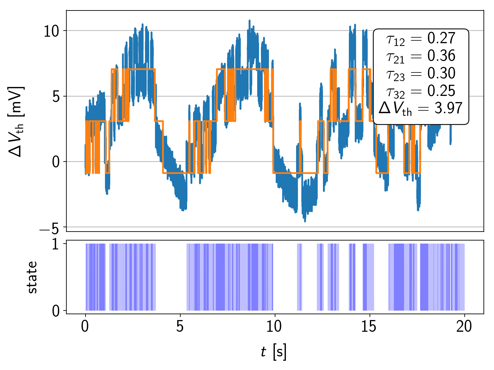
is 3 mV. The orange lines represent the result of the Baum-Welch algorithm without baseline correction. As the Baum-Welch algorithm is sensitive to absolute levels, the noise causes wrong results in terms of the time constants, the offset and .
In the following paragraphs, three different methods for data smoothing, namely local regression or scatterplot-smoothing, basis-spline (B-spline) smoothing and asymmetric least-squares smoothing will be discussed. The answer to the question which of the three baseline estimators should be taken for HMM training highly depends on the signal quality and the trade-off between quality and computational time. A more detailed discussion about different methods for data smoothing can be found in [176] and [177].
Before going into more detail about the proposed methods, a comparison between the results of the baseline estimation algorithms on real measurement data is given in Figure 6.14. The arPLS
algorithm is specifically designed to find the baseline of the data, whereas the LOWESS and B-splines algorithm ( ) delivers least-squares estimates of the local means of the signal. Thus, for the latter two algorithms the RTN signal needs to be removed from the data prior to the baseline fitting.
B-splines were the fastest method of the presented ones, however, they should only be used on measurements with low to medium noise, as the inaccuracies introduced at the boundaries and the knot placements highly depend on the signal noise.
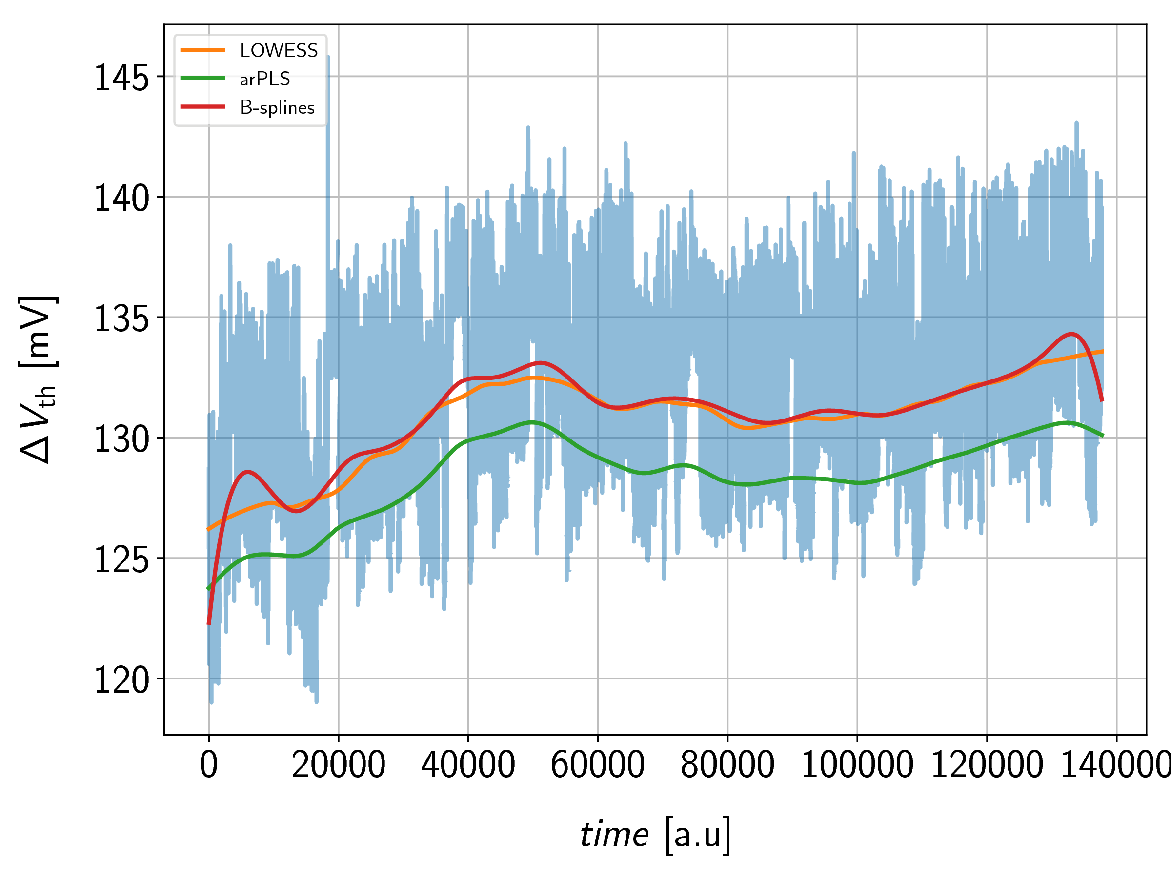
) delivers least-squares estimates of the local means of the signal. Thus, for the latter two algorithms the RTN signal needs to be removed from the data prior to the baseline fitting. The data was taken from real measurements in order to not bias the results by using some analytic drift terms on artificial data.
On the other hand, LOWESS was proven to be the most robust method, delivering decent results for all kind of signals. Despite of being quite slow, just like with the B-spline method, the local mean of the signal is fitted. This makes it necessary to subtract the emissions of the HMM from the measurement signal at every iteration to get a raw estimation of the noisy baseline. That can be a problem as the emissions and the baseline estimation become coupled and potentially can lock up in intermediate results. The mechanism is that emissions get fitted into the baseline, which makes them invisible for further HMM training.
The arPLS method is the only method available to estimate the baseline from the original RTN data (i.e., without subtracting the emissions beforehand). This potentially mitigates the lock-up problem between baseline and emissions mentioned before. However, it also imposes a more severe problem: For slow states, the baseline tends to be pulled towards the signal depending on the choice of the smoothing parameter. When used on the raw baseline of the data mentioned before, it tends to introduce some numerical drift as it then tries to match the baseline of the residual noise after the removal of the emissions. It was also by far the slowest and most numerically unstable method when used on real data and thus is only of limited value for the examined signals.
A robust algorithm for local regression and scatterplot-smoothing was originally proposed in 1979 by William S. Cleveland and later refined by Cleveland and Devlin [178, 179]. The idea is to fit a low-order polynomial to a point based on a subset of the data at each data point. The polynomial is fitted to the subset by a weighted least-squares algorithm with less weight given to points further away from the fitted data point. Each subset thereby is selected by a nearest-neighbor algorithm. The degree of smoothing is usually selected by a parameter which determines the fraction of data points used to fit the local polynomial.
The degree of the polynomial can be chosen freely, however, high-degree polynomials are numerically unstable, computationally expensive and would tend to overfit the data. For these reasons usually first or second order polynomials are used. For a zero-order polynomial, LOWESS falls back to a running mean.
The variant of the LOWESS algorithm used in this work was written by C. Vogel [180] and uses a first-order polynomial. The smoothed value  for the value
  is calculated as the sum of weighted projections of all nearest-neighbor points
  .
.
Here,  is the projection vector calculated from the weighted distances from point to its neighbors. Note that the distances
  ,
,  and
and  have to be given in units of the window size.
The sum of the weighted distances of all neighboring points  within the window
  is
is
The projection factors can then be calculated with:
The weight function  traditionally is the tri-cube weight function:
The biggest advantage of LOWESS over many other methods is that it does not require to find a specific analytic function to fit all the data. This makes it a very flexible tool to fit almost all types of curves for which no proper analytic approximations exist. It can also be used to compute the uncertainty of the fit for model prediction and calibration. Another benefit is the simplicity of the model since the user also only has to provide a value for the smoothing parameter and specify the degree of the local polynomial.
One disadvantage of this method is that rather large, densely sampled datasets are needed in order to produce meaningful results. Another drawback is the fact that no analytic regression function is produced so that the results can easily be shared with the community. Maybe the most severe drawback is the computational cost especially for large datasets, as the regression described above in principle needs to be executed for each data point. This problem can be eased by defining a distance for which the previously fitted value is ‘close enough’ and make regressions only for data points lying at least that distance apart. The values in between are then interpolated linearly.
This method works by fitting a sequence of piecewise polynomial functions to a given dataset. The pieces are defined by a sequence of knots, where for a spline of degree  the spline and its first
  derivatives need to agree at the knots.
Ordinary splines can be represented by a power series of degree for knots [176]
with  being the splines with the coefficients
  ,
,  being the values outside the knots and the notation
Note that usually additional boundary restrictions have to be introduced, since the power series in (6.79) has  parameters to estimate with only observations. One possibility would be to fix the values and their derivatives at the boundaries of the dataset (usually to zero).
Although the representation of splines as power series is well suited to understand the fundamentals of spline representation, they are not very well suited for computation [176]. A much better way is to express them as a linear
combination of basis functions called B-splines. Carl de Boor derived a numerically stable algorithm to construct those B-splines in 1976 [181]. The basic principle is that any spline function of the order on a given sequence of knots can be represented by a linear combination of a set of B-splines.
If the number of knots equals the number of data points the resulting set of splines can be used for interpolating the data between two points. On the other hand, this method can also be used efficiently to smooth a scatterplot if  . The main problem here is the placement of the knots and the treatment of the boundaries which are often cited as the main drawbacks of spline smoothing. The algorithm used in this work is based on the work of Paul Dierckx [177, 182, 183] and is available as the function splrep in the Python library
scipy.interpolate. It automatically selects the number of knots and their positions based on an empirical smoothing parameter
. The main problem here is the placement of the knots and the treatment of the boundaries which are often cited as the main drawbacks of spline smoothing. The algorithm used in this work is based on the work of Paul Dierckx [177, 182, 183] and is available as the function splrep in the Python library
scipy.interpolate. It automatically selects the number of knots and their positions based on an empirical smoothing parameter  which is calculated from the weights provided for each data point.
If the sum of the provided weights is a measure for the inverse of the standard deviation of the signal, the smoothing parameter should be in the interval of  with being the number of points. In Figure 6.14 it can be seen that the results of the B-splines closely resemble those of the LOWESS method except on the boundaries of the signal. It has to be
noted that this method is very sensitive to the placement of the knots, which makes it less robust compared to LOWESS especially for very noisy signals. On the other hand, it is considerably faster and needs fewer points to deliver decent results.
with being the number of points. In Figure 6.14 it can be seen that the results of the B-splines closely resemble those of the LOWESS method except on the boundaries of the signal. It has to be
noted that this method is very sensitive to the placement of the knots, which makes it less robust compared to LOWESS especially for very noisy signals. On the other hand, it is considerably faster and needs fewer points to deliver decent results.
The third and last presented method for baseline estimation is based on a regularized least squares method, where the signal vector  is smoothed by its least squares approximation
  . The method was specifically developed to estimate the baselines in different kinds of spectroscopy data. The objective function to be minimized is defined as [184]
with  being the second order difference matrix of the signal.
The first term of (6.82) expresses the fitness to the data, whereas the second term specifies the amount of smoothing. To identify the regions of the peaks, a weight vector is introduced which can be set to zero at the peak regions if they are known beforehand. This however requires peak finding algorithms which can be difficult to implement especially for noisy data.
The objective function with the diagonalized weight vector  then becomes:
The solution of the minimization problem in (6.84) is given by [184]:
The advantage of this method is that a proper construction of the weight vector allows skipping the peak finding algorithm. At first, this was done Eilers and his peers [185, 186], who simply specified an asymmetry parameter  defined as:
Later, Zhang pointed out that the parameters and need optimization to get adequate results and also that the weights in the baseline region are all the same instead of being set according to the difference of signal and baseline. This was the main motivation to set the weights iteratively based on the current estimate [187].
The iterative procedure stops if the norm of the vector  containing the negative elements of the residuals
  is smaller than a certain fraction of the norm of . The problem with these methods is that the values below the baseline in the non-peak regions are considerably stronger weighted compared to those above. This results in an underestimation of the baseline and thus an overestimation of the peaks in the iterative procedure.
To correct for this error, the arPLS method was suggested in [184] which uses a more symmetric way to define the weights using a generalized logistic function defined by the mean value and the standard deviation of .
The logistics function gives nearly the same weights for all values below the baseline estimate up to a distance  from the mean. At a distance
  from the mean, the weights are already practically zero. Figure 6.15 depicts the logistics function in units of
  and .
and .
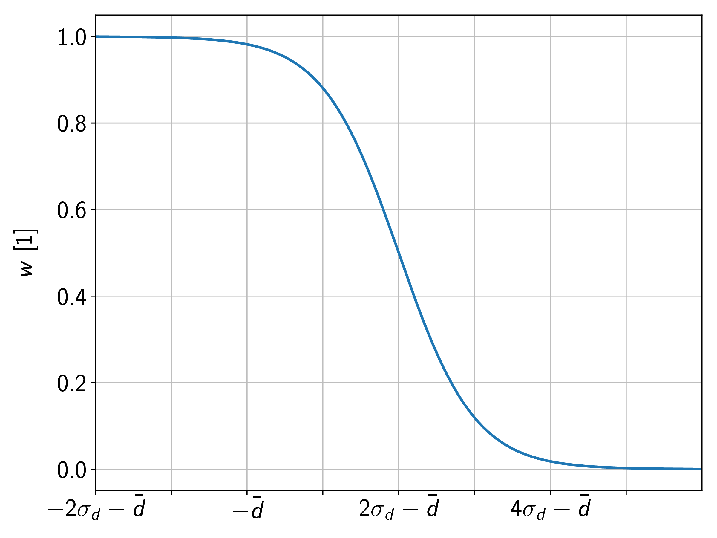
from the mean. At a distance from the mean, the weights are already practically zero.
From the three investigated weight functions, on average the logistic function delivered the most reliable results across the measurement data and thus should be used for baseline estimation.
The main benefit of arPLS compared to LOWESS and B-splines is that it can be used on the original data since it is specifically designed to follow the baseline of the signal. The other two methods settle somewhere around the local mean of the signal. Thus they cannot be used on the measurement signal as they are.
The drawbacks of arPLS are the size of the sparse matrix system to solve which is equivalent to the number of data points. Also, the parameter for smoothing scales with the signal length and was found to be numerically unstable above a certain threshold. Whether this is due to the accuracy of the used solver or the numeric resolution of the datatypes needs to be investigated. Another drawback is the computation time and the number of iterations
needed to reach a stable result. While a single iteration was approximately two times slower than a LOWESS iteration, the algorithm needs at least five iterations to converge, assuming a stable solution. This makes it ten times slower compared to LOWESS which only needs one to two iterations if the data is
sufficiently dense.
On the following pages, the implemented HMM library will be tested with sampled data coming from a simulated system of two defects with known properties (for details on the HMM implementation see Appendix A). The simulated data is varied by different means and given to an independent system with the same structure but different initial conditions for training. It is thus possible to check for the robustness of the implementation by comparing the training results to the known system, which would not be possible when using real measurement data.
Note that up to this point, no assumptions regarding the physics or structure of the defects except the Markov property were made. This is quite convenient, since choosing a physical model beforehand could lead to biased results with respect to the time constants.
For the sample system, one four-state defect ‘A’ containing one thermal state is combined with a two-state defect ‘B’. The Markov chain of both defects as well as their RTN signal is given in Figure 6.16.

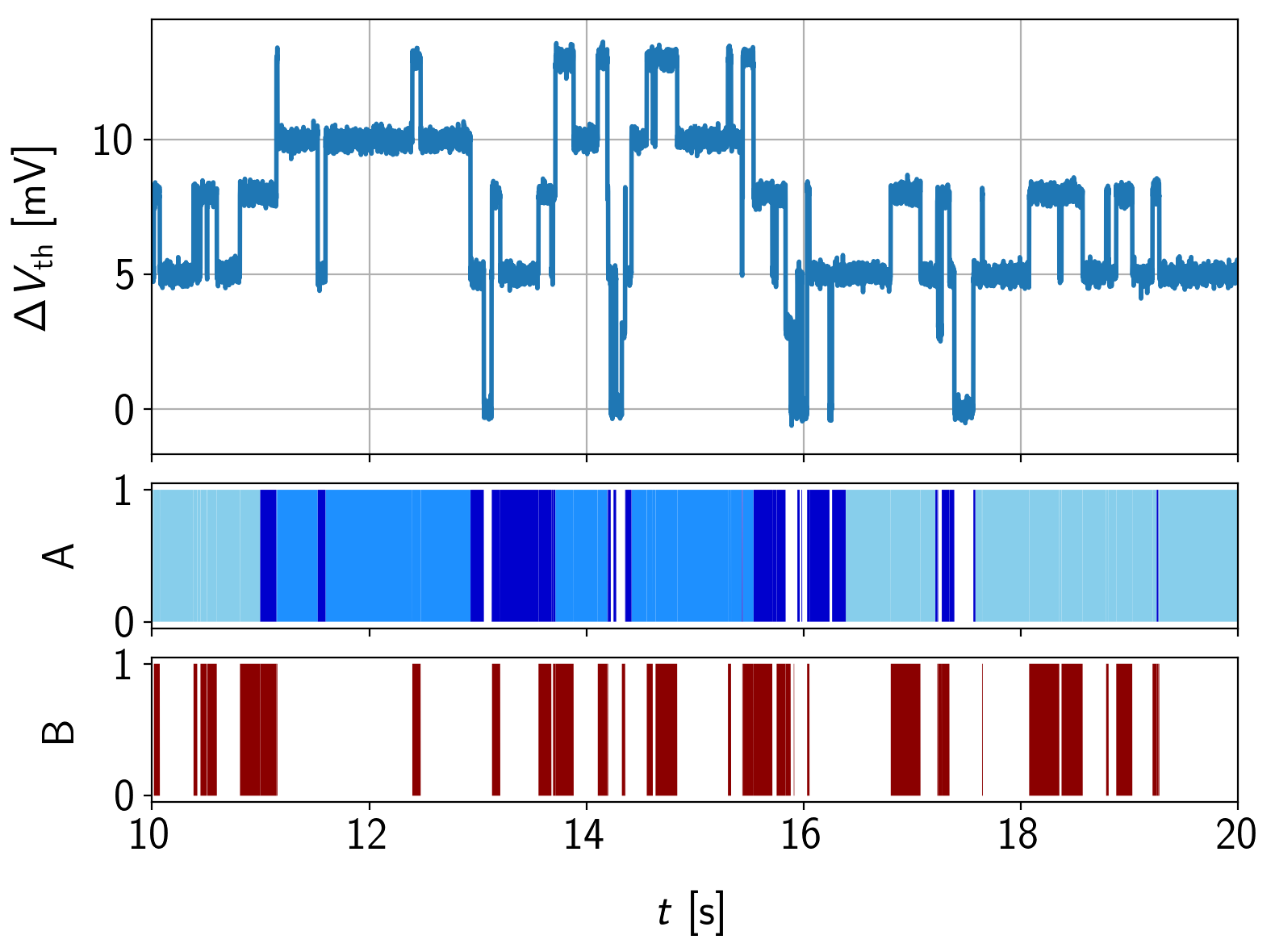
, negative if in state  or and double negative in state
  . The step heights are 5 mV and 3 mV.
The first thing to investigate is how many transitions are actually necessary to obtain a reliable result. In order to do that, the confidence intervals of the exponential distribution over the number of transitions are calculated. Given the maximum likelihood estimate of the characteristic time-constant  and the number of expected transitions , the
  confidence intervals are given by [188]:
where  is the -percentile of the chi-squared distribution with
  degrees of freedom. The results in Figure 6.17 show that about 19 transitions are needed within a
  confidence interval in order to obtain an maximum error of
  . For a ninety-percent confidence interval, this value already goes up to 46 (dashed lines). For a maximum error of ten percent, the minimum number of transitions are already 120 for the one-sigma interval and 315 for the ninety-percent interval (solid lines).
These numbers can also be used to estimate measurement times for simple RTN signals. Note that for multi-state defects, the number of observed transitions within a time interval scales with the first-passage times of the defect’s state (imagine a three-state defect with a slow state on top of a fast one).
The red area in Figure 6.17 shows the Normal approximation of the one-sigma confidence interval of the exponential distribution. It can be seen that in this case, the confidence intervals only diverge significantly from the chi-squared distribution if there are less than five transitions. However, for the 90 % confidence intervals, the number of transitions to obtain a similar well-approximated result is at least one order of magnitude above that value, meaning that the quality of the approximation largely depends on the chosen confidence interval. The HMM library thus routinely calculates the 90 % confidence intervals using equation (6.89).
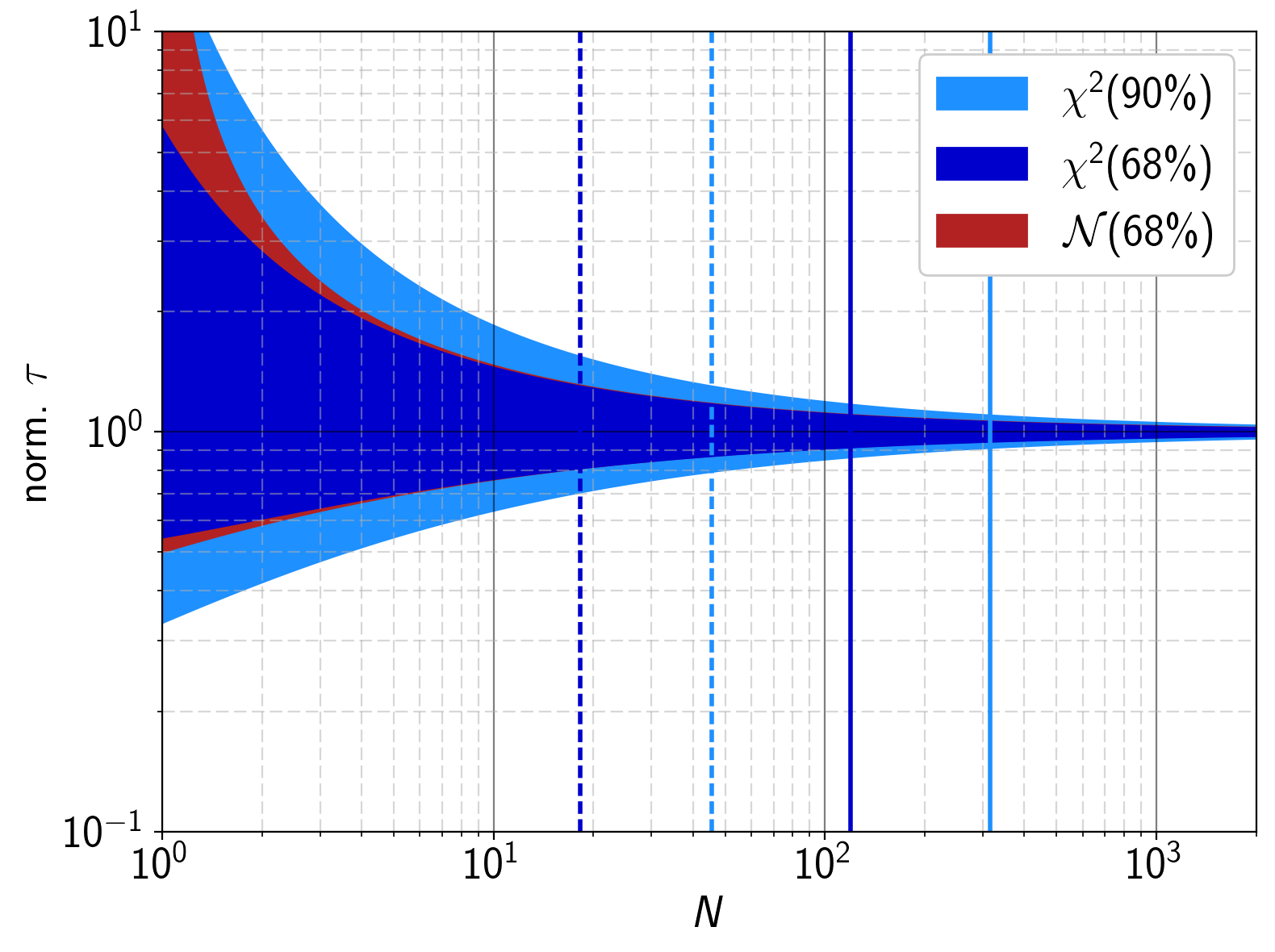
, for the solid lines the error is within  . The shaded red area is the one-sigma confidence interval in a Normal approximation.
For the following simulation study, the initial parameters for ,  and the simulated measurement signal were chosen randomly with 100 different seeds. The first thing checked is the sensitivity of the HMM library to the initial conditions in terms of the characteristic times and . The initial and final time constants of each defect were normalized and binned into a single histogram as shown at the upper part of Figure 6.18. For both defects, the model most of the
time converges towards the proper solutions, even with a quite broad distribution of the initial values.
and the simulated measurement signal were chosen randomly with 100 different seeds. The first thing checked is the sensitivity of the HMM library to the initial conditions in terms of the characteristic times and . The initial and final time constants of each defect were normalized and binned into a single histogram as shown at the upper part of Figure 6.18. For both defects, the model most of the
time converges towards the proper solutions, even with a quite broad distribution of the initial values.
The lower part of Figure 6.18 gives the sensitivity to the step heights of the defects. As with the time constants, the sensitivity to variations of the initial conditions is very low. It should be noted that as mentioned in Section 6.7, the Baum-Welch algorithm converges towards a local maximum. This can be seen especially in the scatterplots for the step heights where distinct secondary peaks in the histograms show up. They are, however, quite small compared to the maximum and thus are not considered as a serious problem.
Another issue to be mentioned is that the initial values for were constrained in such a way that the initial value of defect ‘A’ with a nominal value of 5 mV had to have a larger value than defect ‘B’ (3 mV) and defect ‘B’ had to be smaller than the nominal value of defect ‘A’. This helps to maintain the structure of the system and helps to find the
proper local minimum in the parameter space. On a side note, it has to be mentioned that some of the seeds delivered impossible solutions having a log-probability of  . This is a well-known issue for the MAP path decoding used in this work. These solutions were filtered from the results before post-processing of the data.
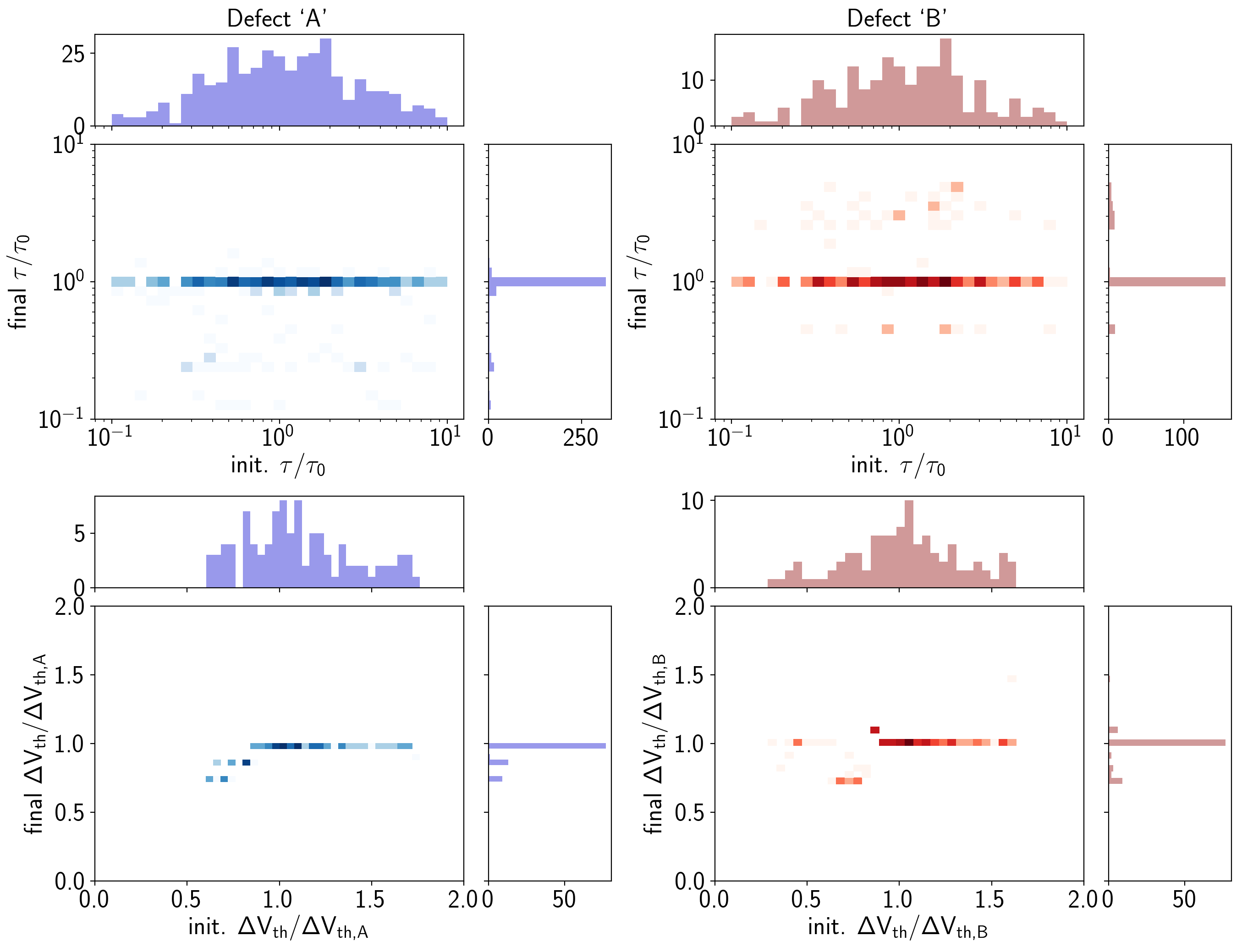
. Although quite broad normal distributions were chosen in both cases, the solutions converged towards the correct values nearly all of the time.
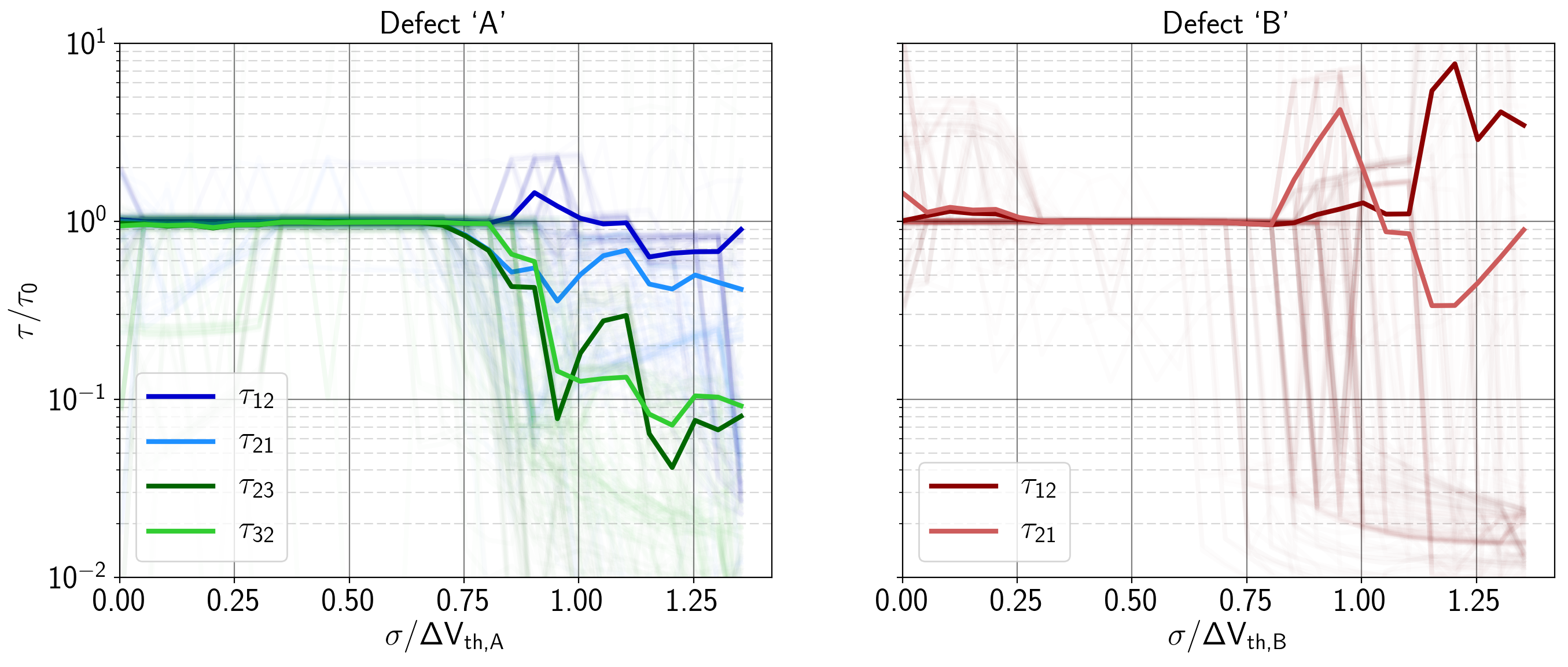
The next property investigated was the sensitivity of the training results regarding (simulated) external measurement noise. For that purpose, Gaussian noise with different values of  was added to the measurement signal. Despite some of the seeds converging to different solutions in Figure 6.19 (faint traces), it can be seen that the weighted average (with the weights being )
of the time constants are very close to their appropriate values up to about a signal to noise ratio of about 0.75, quickly diverging for values above that.
was added to the measurement signal. Despite some of the seeds converging to different solutions in Figure 6.19 (faint traces), it can be seen that the weighted average (with the weights being )
of the time constants are very close to their appropriate values up to about a signal to noise ratio of about 0.75, quickly diverging for values above that.
This can easily be explained by the fact that considering an interval of about  , the noise level at that point on average becomes larger than the step height. The point at which the solutions begin to degrade could probably still be pushed a bit further by broadening the statistics (i.e. expanding the cumulated measurement time). Considering that the simulations were sampled at
1 kHz for 1 ks (i.e.,
, the noise level at that point on average becomes larger than the step height. The point at which the solutions begin to degrade could probably still be pushed a bit further by broadening the statistics (i.e. expanding the cumulated measurement time). Considering that the simulations were sampled at
1 kHz for 1 ks (i.e.,  samples), for a maximum time constant of 2 s (see Figure 6.16), the effect is thought to be quite small.
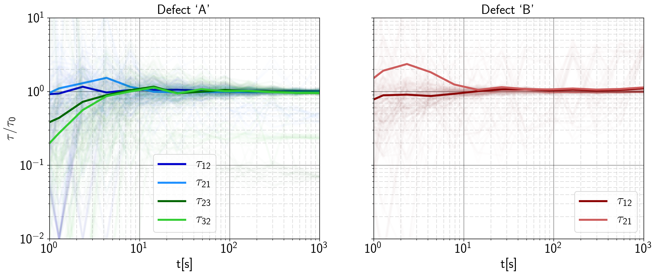
The dependence of the solutions over measurement time is given in Figure 6.20 for  and a sampling frequency of 1 kHz. Except for measurement times below 10 s, the training results are close to their real values on average. The uncertainty of the solutions naturally increases at lower times as there are fewer transitions contributing to the solution within one measurement
window. Above
and a sampling frequency of 1 kHz. Except for measurement times below 10 s, the training results are close to their real values on average. The uncertainty of the solutions naturally increases at lower times as there are fewer transitions contributing to the solution within one measurement
window. Above  or a few transitions for the slowest state, the statistics for that system seems to be sufficient (see also Figure 6.17).
It should be said that the intuitive feeling that the minimum number of observed transitions for a given system is the measurement time over the slowest capture or emission time is only valid for systems consisting of two-state defects. This is because for more complicated cases, the first passage times of the defect’s
Markov chains determine the observed number of transitions. As an example, a three-state defect with a  will hardly be able to reach state 3 at all.
Also, the number of different simulations help to effectively increase the statistics in a way that the cumulated time increases with every different seed. Although each training was done independently on one simulated trace, the median values of the results naturally follow the cumulated times.
For real devices, another complication arises due to the broad distributions of capture and emission times observed in GaN devices [6, 44]. Faster sampling rates or longer measurement times will always result in additional defect transitions, which had not been within the measurement window before. With other words, the faster the sampling, the more of the fast defects can be seen and the longer the measurement the more of the slow defects can be seen.
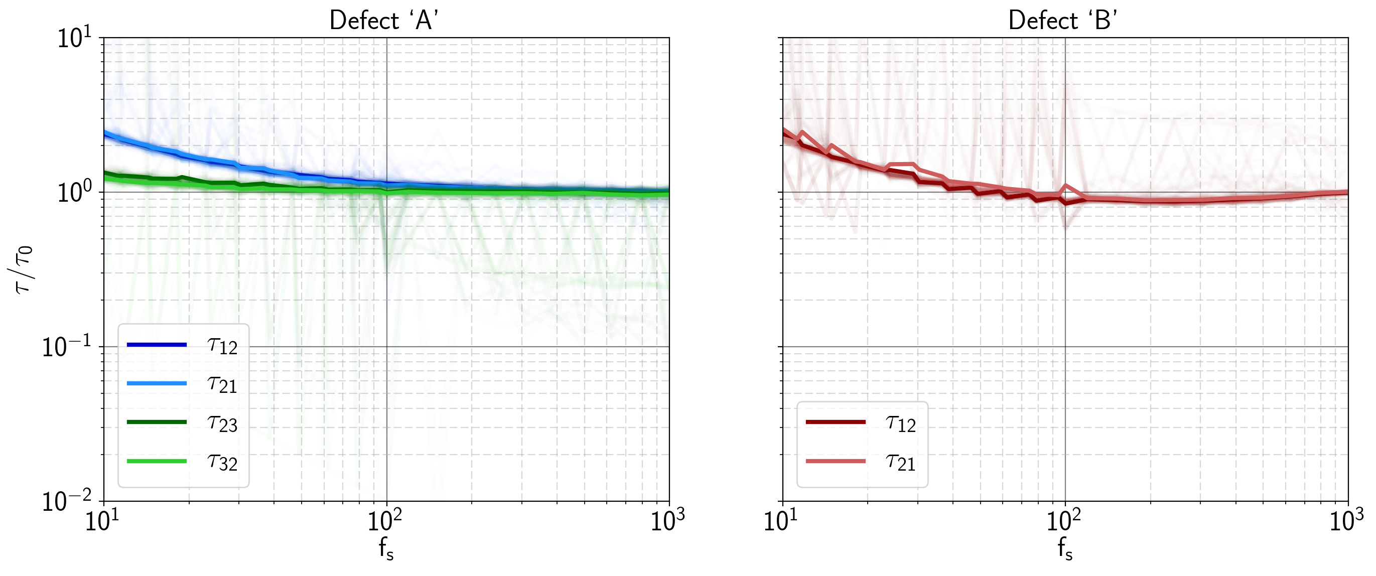
The next test was done by comparing the results for different sampling frequencies. The measurement time was chosen to be 1 ks with a Gaussian noise of 0.5 mV. Surprisingly, the results in Figure 6.21 were consistent down to 100 Hz, which already is equivalent to the emission time of the fastest state. This finding can maybe be explained by the fact that emissions faster than the sampling frequency will be partly truncated at the sampling time and partly be sampled out of the signal (depending on the point of sampling). The lower part of an exponential distribution centered around the sampling frequency thus will be seen as an additional peak at the minimum time, not changing the overall expectation value of the distribution very much.
On the other hand, the induced distortions and aliasing effects could potentially obfuscate the real structure of the Markov chain as well as the training results. It is thus recommended to maintain a sufficient Nyquist margin when downsampling data or setting up measurements.
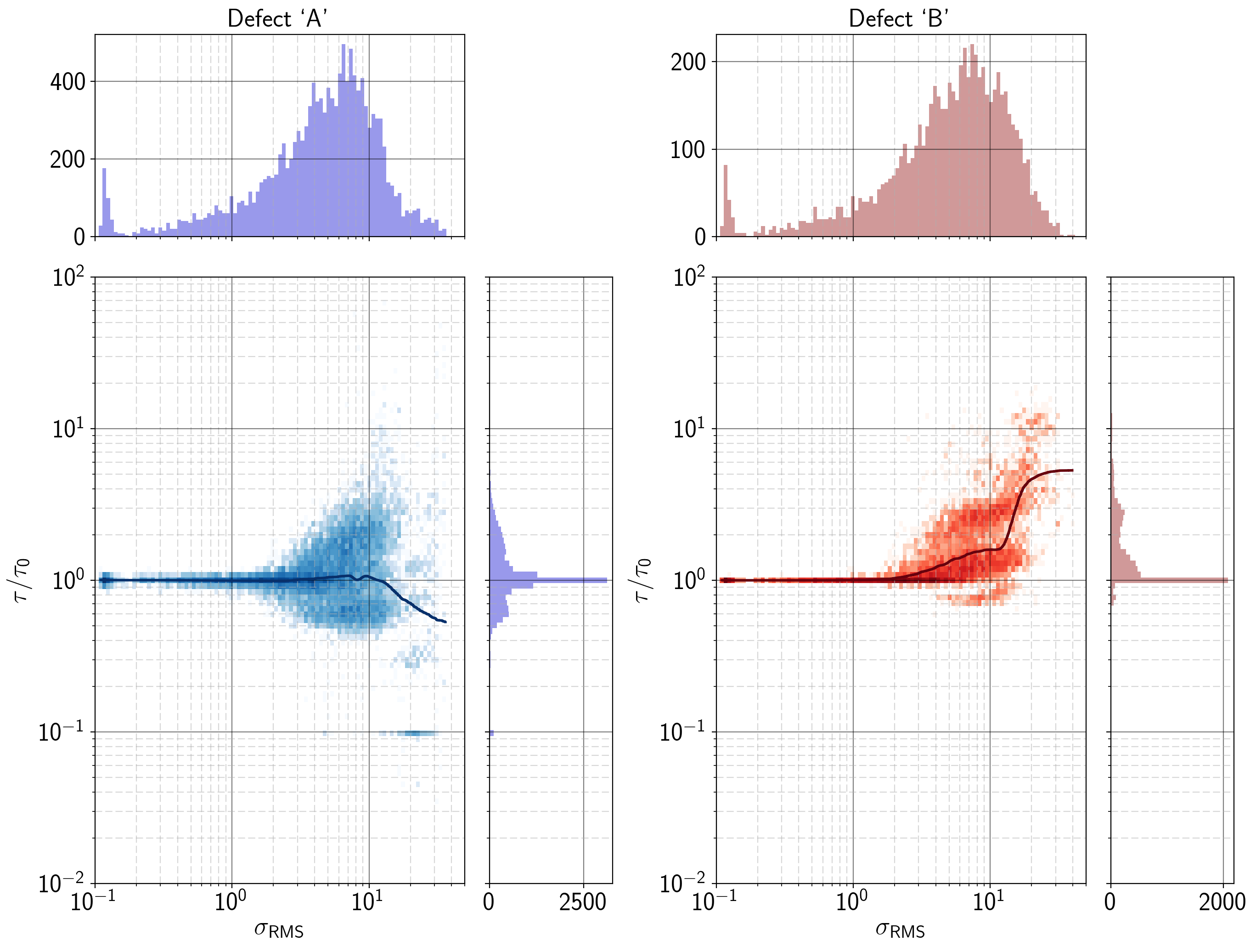
The last benchmark was to test the robustness of the baseline fitting algorithm of the HMM library. For that purpose, random walks with different amplitudes per step were generated in order to obtain as many different long-term drift conditions as possible. To further complicate the problem, an additional 50 Hz signal with Gaussian spectrum was added to the drift signal. The Gaussian noise of the samples was again 0.5 mV.
The main motivation of using random walks is to eliminate biased results based on the analytic form of the drift signal (i.e., by using combinations of polynomial or exponential terms for simulating drift). As a measure of severity of the drift the RMS of the baseline was calculated, despite not being ideal as for example also the number of turning points or the maximum gradient of the signal could influence baseline extraction.
In Figure 6.22, the cumulated 2D-histogram of the normalized times versus the RMS values of the drift signal are shown. The solid line was calculated with the LOWESS method and thus gives the center of mass across the density plot. The density plot is printed on a logarithmic color scale in order to show the spreading of the results with increasing drift which was almost not visible on a linear scale.
The center of mass resembles the real values closely up to a value of around  . After that, the solutions start to degrade quickly. A partial explanation of that behavior would be that the tails of the histogram of drift values is reached, which leads to more statistical uncertainty due to the small sample size. On the other hand, the initial guess of the forward-backward algorithm (which is
done with a constant offset) on average covers fewer emissions. The uncovered emissions are then used wrongly to calculate the baseline signal which in turn forces the HMM into wrong solutions.
. After that, the solutions start to degrade quickly. A partial explanation of that behavior would be that the tails of the histogram of drift values is reached, which leads to more statistical uncertainty due to the small sample size. On the other hand, the initial guess of the forward-backward algorithm (which is
done with a constant offset) on average covers fewer emissions. The uncovered emissions are then used wrongly to calculate the baseline signal which in turn forces the HMM into wrong solutions.
A definitive answer to the question whether one of those mechanisms is dominant is hard to estimate. In any case, given a fixed set of measurements, the only way to obtain robust results is to train the model with as many different initial conditions as possible.
 can be understood by the limits imposed by the measurement time and the sampling frequency for the different defects.


![(6.46) \begin{equation} \alpha _t(i)=\left [\sum _{j=0}^{N-1}{\alpha _{t-1}(j)k_{ji}}\right ]b_i(\obs _t) \end{equation}](images/image-609.svg)


![(6.51) \begin{equation} \hat q(t) = \underset {i}{\mathrm {argmax}}[\gamma _t(i)] \eqlabel {rtnextract:hmm:qt} \end{equation}](images/image-636.svg)
![(6.52) \begin{equation} Q(\lambda ,\hat \lambda ) = \sum _X{P(X|\obs ,\lambda )\mathrm {log}[P(\obs ,X|\hat \lambda )]} \eqlabel {rtnextract:hmm:Q} \end{equation}](images/image-640.svg)
![(6.53) \begin{equation} \underset {\hat \lambda }{\mathrm {max}}[Q(\lambda ,\hat \lambda )] \rightarrow P(\obs |\hat \lambda ) \geq P(\obs |\lambda ). \eqlabel {rtnextract:hmm:maxQ} \end{equation}](images/image-643.svg)


![(6.59) \begin{equation} \underline {\bm {k}} = \begin{bmatrix}[1.5] k^\mathrm {B}_{11}k^\mathrm {A}_{11} & k^\mathrm {B}_{11}k^\mathrm {A}_{12} & k^\mathrm {B}_{12}k^\mathrm {A}_{11} & k^\mathrm {B}_{12}k^\mathrm
{A}_{12}\\ k^\mathrm {B}_{11}k^\mathrm {A}_{21} & k^\mathrm {B}_{11}k^\mathrm {A}_{22} & k^\mathrm {B}_{12}k^\mathrm {A}_{21} & k^\mathrm {B}_{12}k^\mathrm {A}_{22}\\ k^\mathrm {B}_{21}k^\mathrm {A}_{11} & k^\mathrm
{B}_{21}k^\mathrm {A}_{12} & k^\mathrm {B}_{22}k^\mathrm {A}_{11} & k^\mathrm {B}_{22}k^\mathrm {A}_{12}\\ k^\mathrm {B}_{21}k^\mathrm {A}_{21} & k^\mathrm {B}_{21}k^\mathrm {A}_{22} & k^\mathrm {B}_{22}k^\mathrm {A}_{21}
& k^\mathrm {B}_{22}k^\mathrm {A}_{22} \end {bmatrix} \eqlabel {rtnextract:hmm:multi} \end{equation}](images/image-684.svg)
![(6.60) \begin{equation} \mat {\delta }^\mathrm {A}_{1} = \begin{bmatrix}[1.5] 1 & 1 & 1 & 1\\ 0 & 0 & 0 & 0\\ 1 & 1 & 1 & 1\\ 0 & 0 & 0 & 0 \\ \end {bmatrix},\‚\mat {\delta }^\mathrm
{A}_{2} = \begin{bmatrix}[1.5] 0 & 0 & 0 & 0\\ 1 & 1 & 1 & 1\\ 0 & 0 & 0 & 0 \\ 1 & 1 & 1 & 1\\ \end {bmatrix} \eqlabel {rtnextract:hmm:masks} \end{equation}](images/image-685.svg)
![(6.61) \begin{equation} {k}^\mathrm {A}_{ij} = \sum {\mat {k}\left [\mat {\delta }^\mathrm {A}_{i}\cdot \mat {\delta }^{\mathrm {A}^\mathrm {T}}_{j}\right ]} \eqlabel {rtnextract:hmm:mask} \end{equation}](images/image-690.svg)
![(6.62) \{begin}{align} {k}^\mathrm {A}_{12} = & \sum {\mat {k}\left [\mat {\delta }^\mathrm {A}_{1}\cdot \mat {\delta }^{\mathrm {A}^\mathrm {T}}_{2}\right ]}\notag \\ = & \sum { \begin{bmatrix}[1.5] k^\mathrm
{B}_{11}k^\mathrm {A}_{11} & k^\mathrm {B}_{11}k^\mathrm {A}_{12} & k^\mathrm {B}_{12}k^\mathrm {A}_{11} & k^\mathrm {B}_{12}k^\mathrm {A}_{12}\\ k^\mathrm {B}_{11}k^\mathrm {A}_{21} & k^\mathrm {B}_{11}k^\mathrm {A}_{22}
& k^\mathrm {B}_{12}k^\mathrm {A}_{21} & k^\mathrm {B}_{12}k^\mathrm {A}_{22}\\ k^\mathrm {B}_{21}k^\mathrm {A}_{11} & k^\mathrm {B}_{21}k^\mathrm {A}_{12} & k^\mathrm {B}_{22}k^\mathrm {A}_{11} & k^\mathrm
{B}_{22}k^\mathrm {A}_{12}\\ k^\mathrm {B}_{21}k^\mathrm {A}_{21} & k^\mathrm {B}_{21}k^\mathrm {A}_{22} & k^\mathrm {B}_{22}k^\mathrm {A}_{21} & k^\mathrm {B}_{22}k^\mathrm {A}_{22} \end {bmatrix} \cdot \begin{bmatrix}[1.5] 0
& 1 & 0 & 1\\ 0 & 0 & 0 & 0\\ 0 & 1 & 0 & 1\\ 0 & 0 & 0 & 0 \\ \end {bmatrix} } \\ = & \sum { \begin{bmatrix}[1.5] 0 & k^\mathrm {B}_{11}k^\mathrm {A}_{12} & 0 & k^\mathrm
{B}_{12}k^\mathrm {A}_{12}\\ 0 & 0 & 0 & 0\\ 0 & k^\mathrm {B}_{21}k^\mathrm {A}_{12} & 0 & k^\mathrm {B}_{22}k^\mathrm {A}_{12}\\ 0 & 0 & 0 & 0 \end {bmatrix} } = k^\mathrm {B}_{11}k^\mathrm {A}_{12} +
k^\mathrm {B}_{12}k^\mathrm {A}_{12} + k^\mathrm {B}_{21}k^\mathrm {A}_{12} + k^\mathrm {B}_{22}k^\mathrm {A}_{12} \notag \{end}{align}](images/image-692.svg)


![(6.68) \{begin}{align} \hat {\sigma }^2_{\mathrm {p}}(i) & = \frac {\sum _j{\big [\Gamma _j(i)-1\big ]\sigma ^2_j(i)}}{\big [\sum _j{\Gamma _j(i)}\big ]-1} + \frac {\sum _j{\Gamma _j(i)\big [\hat \mu _j(i) - \hat {\mu }_\mathrm
{p}(i)\big ]^2}}{\big [\sum _j{\Gamma _j(i)}\big ]-1}. \eqlabel {rtnextract:hmm:sigma_pooled} \{end}{align}](images/image-718.svg)
![(6.69) \{begin}{align} \hat {\sigma }^2_{\mathrm {p}}(i) & = \frac {\sum _j{\big [\big (\Gamma _j(i)-1\big )\sigma ^2_j(i)} + \Gamma _j(i)\hat \mu ^2_j(i)\big ] - \big [\sum _j{\Gamma _j(i)}\big ]\hat {\mu }^2_\mathrm
{p}(i)}{\big [\sum _j{\Gamma _j(i)}\big ]-1}. \eqlabel {rtnextract:hmm:sigma_pooled2} \{end}{align}](images/image-720.svg)


![(6.72) \begin{equation} \mat {Q} = \big \{[\mathbin {\textcolor {red}{0}}\ \mathbin {\textcolor {blue}{0}}],\ [\mathbin {\textcolor {red}{0}}\ \mathbin {\textcolor {blue}{1}}],\ [\mathbin {\textcolor {red}{1}}\ \mathbin {\textcolor
{blue}{0}}],\ [\mathbin {\textcolor {red}{1}}\ \mathbin {\textcolor {blue}{1}}],\ [\mathbin {\textcolor {red}{2}}\ \mathbin {\textcolor {blue}{0}}],\ [\mathbin {\textcolor {red}{2}}\ \mathbin {\textcolor {blue}{1}}]\big \}. \eqlabel
{rtnextract:hmm:chargeset2} \end{equation}](images/image-734.svg)

![(6.74) \begin{equation} \begin{bmatrix}[1.3] \hat {\sigma }_0^2 \\ \hat {\sigma }_1^2 \\ \hat {\sigma }_2^2 \\ \hat {\sigma }_3^2 \\ \hat {\sigma }_4^2 \\ \hat {\sigma }_5^2 \\ \end {bmatrix} = \begin{bmatrix} 0 & 0\\ 0 &
1\\ 1 & 0\\ 1 & 1\\ 1 & 0\\ 1 & 1\\ \end {bmatrix} \cdot \begin{bmatrix}[1.3] \sigma _\mathrm {A}^2 \\ \sigma _\mathrm {B}^2 \end {bmatrix} + \sigma _\mathrm {off}^2 \eqlabel {rtnextract:hmm:charge_sigma} \end{equation}](images/image-739.svg)


![(6.77) \begin{equation} p_{ij} = w_j \bigg [ 1 + \frac {(x_i - \hat x)(x_j - \hat x)}{\sum _k{w_{k}(x_k - \hat x)^2}}\bigg ] \eqlabel {rtnextract:hmm:lowess_pij} \end{equation}](images/image-762.svg)