The procedure presented in the previous section can easily be generalized to more than two states. The Master equation for state  is given by the probabilities to go from state to state
  together with the probability to stay in state [153]:
From those probabilities, the Master equation is again obtained analogous to equation (6.10) using  .
.
Since the charge has to be in one of the states, from  equations, only
  are independent from each other. The PDF of the first passage times for multi state defects can again be derived from the solution of the Master equation. For a three-state defect this is done in [110], while [153] gives more general approaches to derive analytic expressions for that problem in Chapter 6. In principle, the same procedure as presented in Section 6.2 can be used to to derive the equilibrium first passage times for neighbouring states, if the correct occupancies are inserted. For non-neighbouring states, the PDFs are the normalized differences of exponential distributions, where the
faster defect truncates the distribution of the slower defect [110]. Since both of the extraction methods presented in Sections 6.6 and 6.7 do not rely on the knowledge of the PDFs, the analytic expressions are omitted at this point.
are independent from each other. The PDF of the first passage times for multi state defects can again be derived from the solution of the Master equation. For a three-state defect this is done in [110], while [153] gives more general approaches to derive analytic expressions for that problem in Chapter 6. In principle, the same procedure as presented in Section 6.2 can be used to to derive the equilibrium first passage times for neighbouring states, if the correct occupancies are inserted. For non-neighbouring states, the PDFs are the normalized differences of exponential distributions, where the
faster defect truncates the distribution of the slower defect [110]. Since both of the extraction methods presented in Sections 6.6 and 6.7 do not rely on the knowledge of the PDFs, the analytic expressions are omitted at this point.
Typical candidates for multistate defects are three-state defects producing two or three level anomalous RTN [108, 112, 113], see also Section 4.2.1. In the case of two-level anomalous RTN as seen in Figure 6.3, the third state possesses the same charge state as the second one. Such states are attributed to a structural relaxation of the defect in the NMP four-state model and will be referred to as thermal states throughout the remainder of this work. There is no straight-forward way to determine a thermal state from the measurements with the histogram methods described in Section 6.6. With respect to Markov models they are also called tied states because they share the same emissions (and thus the same PDF for the emissions) with the state they are tied to.

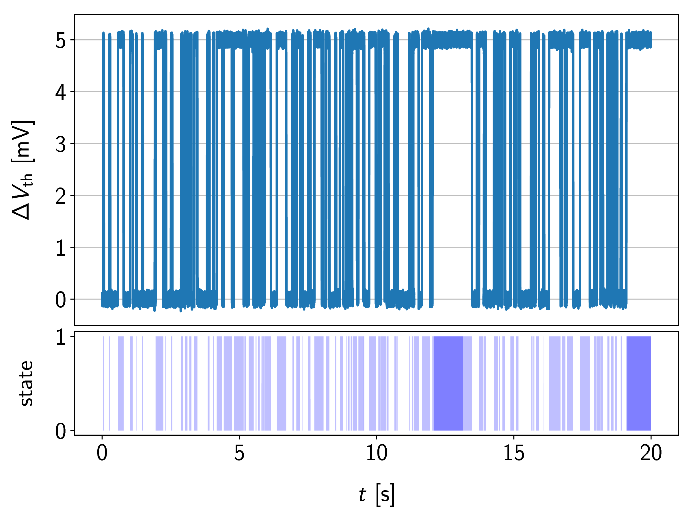
 and negative if in state
  or
or  . Right: Simulated emissions of the three-state defect for
  and
and  . Note that there is no straight-forward way to determine the thermal state directly from measurements. The simulations were done with the Hidden Markov library presented in Section 6.7, with a small
amount of Gaussian noise added to the emissions.
. Note that there is no straight-forward way to determine the thermal state directly from measurements. The simulations were done with the Hidden Markov library presented in Section 6.7, with a small
amount of Gaussian noise added to the emissions.
An example for an even more complex RTN signal commonly called three-level anomalous RTN, is given in Figure 6.4. Here the Markov state is charged negatively, while the states  and
and  are charged double-negatively. Again, the states and cannot be separated easily, because they share the same charge state.

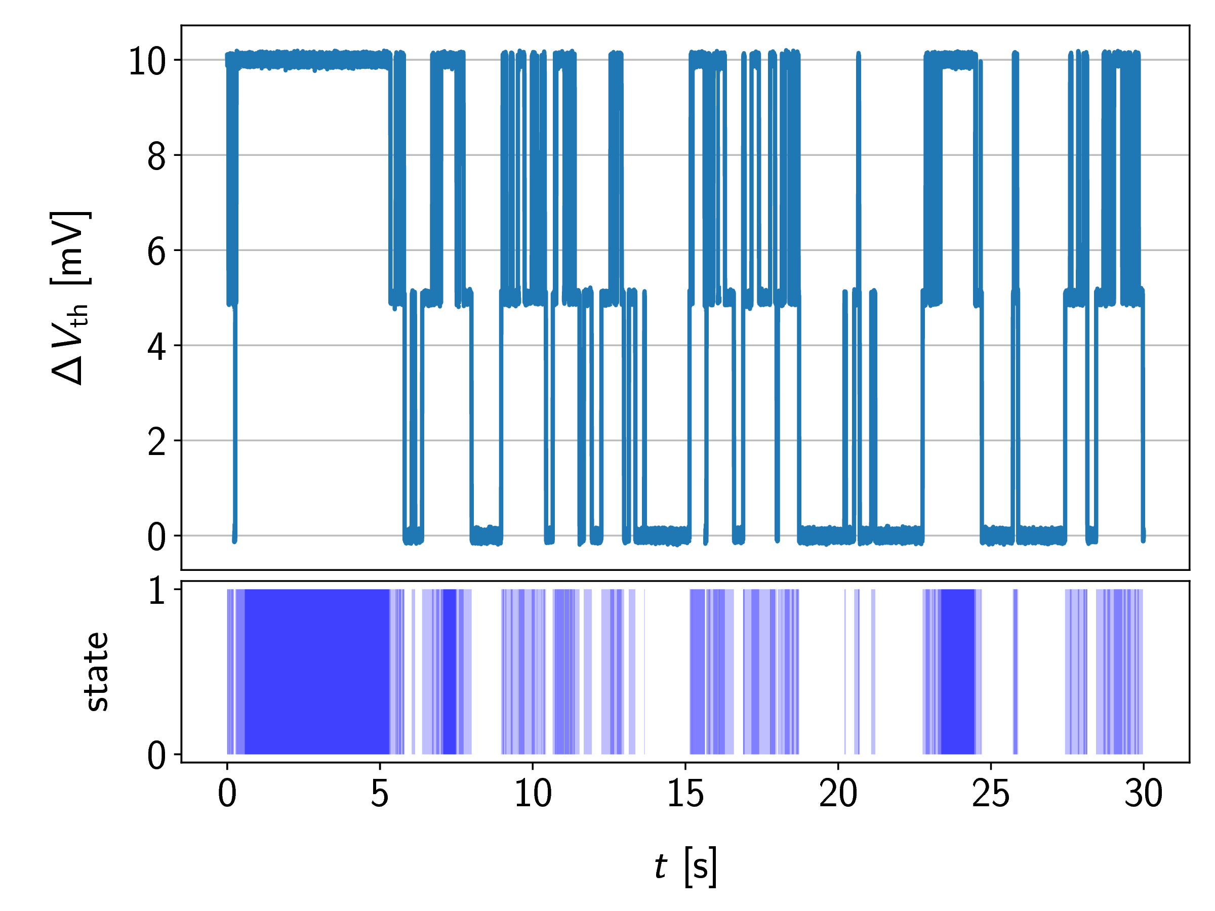
, negative if in state and double negative in the states and . Right: Simulated emissions of the three-level defect for  ,
,  and
and  . The simulations were done with the Hidden Markov library presented in Section 6.7, with a small amount of Gaussian noise added to the emissions.


