Charge Trapping and Single-Defect Extraction in Gallium-Nitride Based MIS-HEMTs

6.6 Histogram-Based Methods

In single defect measurements, defects are commonly identified by clustering the observed step heights into spectral maps, see Section 4.2 and [110, 115–117, 158]. The most important difference in obtaining the stochastic times between TDDS and RTN measurements is that for TDDS measurements, emission times of a defect are equal to the points in time of the steps in the recovery traces. That means the clusters can be obtained in a rather straight-forward manner by printing the step-height distribution versus the observed emission times to a two-dimensional histogram (see Figure 4.4). For RTN signals, either the probability distribution of the signal amplitude when being in a certain state or the time differences between adjacent capture and emission events have to be calculated. The extraction of those can be rather challenging, especially for more complex RTN signals. Such signals can either be composed of defects with multiple emissions or emissions from different defects possessing similar step-heights [AGC5]. The most common conventional methods to extract time constants directly from measurements are done from histograms of the signal amplitudes or so-called lag plots, which are correlation plots between neighboring measurement samples. The main problem of those two methods is that they are quite prone to measurement noise and tend to miss smaller, non-dominant defects (i.e. the minor modes of the multimodal distributions) due to noise. They also rely on the absolute values of the measurement signal, which makes them sensitive to long-term drift on the RTN signal [133, 159, 160].

After a brief introduction to the histogram method in Section 6.6.1 and the lag plot method in Section 6.6.2, Section 6.6.3 presents a modified version of the histogram method for the extraction of time constants in TDDS measurements [116].

6.6.1 Amplitude Histograms

A method which makes use of the signal amplitude histograms to derive step heights and time constants of RTN producing defects was first introduced by Yuzhelevski and co-authors in 2000 [160]. In order to calculate the defect properties, the measurement values are directly binned into a histogram. The step-height(s) (math image) can in principle be derived directly from the observed amplitude distributions. If the number of samples is sufficiently large and the peaks of the Gaussian distributions are well separated, the capture and emission times of the (presumably) two-state defects can be calculated with the histogram areas $A_\mathrm {L}$ and $A_\mathrm {H}$ , the bin size $\mathrm {\Delta U}$ of the Gaussians as well as the number of transitions $k$ and the sampling time $\mathrm {\Delta }t$ [160] using

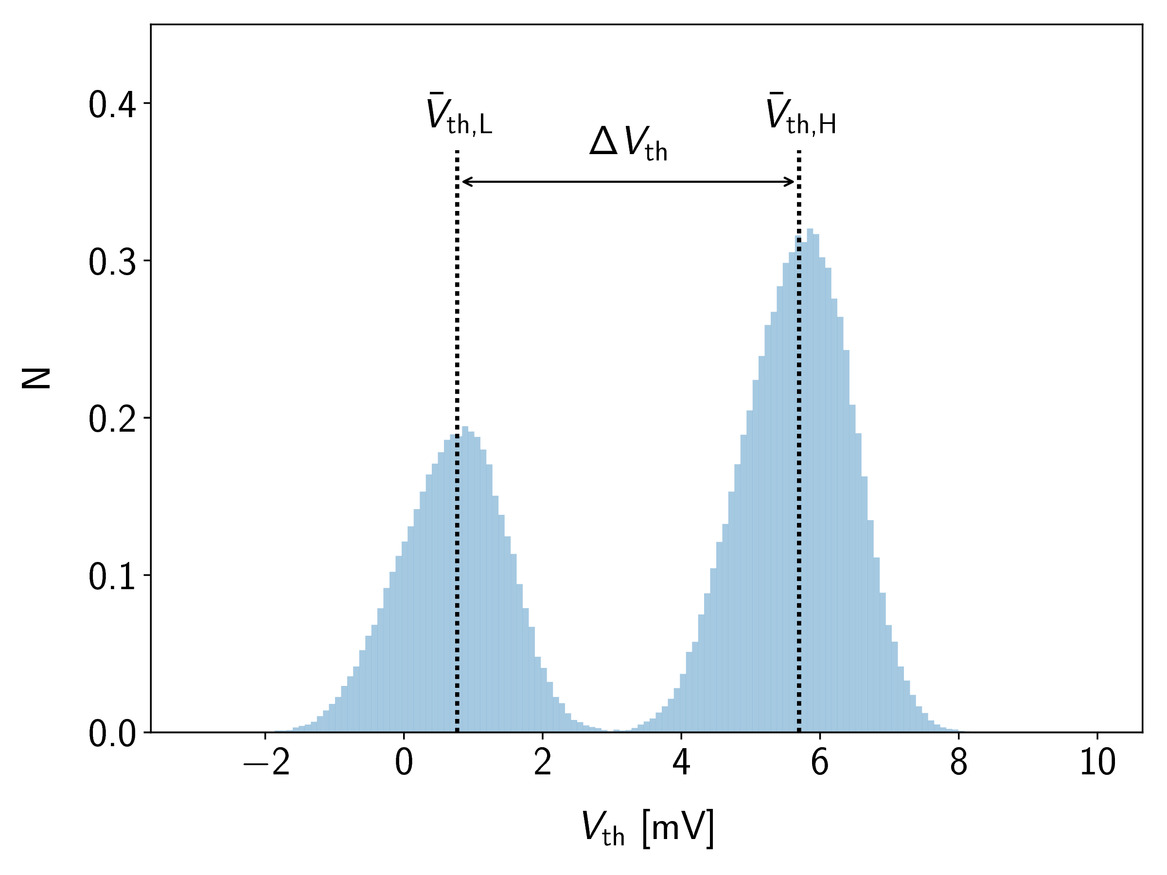
$(6.366.37) \{begin}{align} \tau _\mathrm {c} & = \frac {2}{k} \frac {A_\mathrm {L}}{\mathrm {\Delta U}}\mathrm {\Delta }t,\\ \tau _\mathrm {e} & = \frac {2}{k} \frac {A_\mathrm {H}}{\mathrm {\Delta U}}\mathrm {\Delta }t. \eqlabel {rtnextract:tauHist} \{end}{align}$

An example of a simulated RTN trace together with the resulting amplitude histogram are given in Figure 6.7. In general, for each (math image) level of the combined system, one Gaussian distribution will be present in the histogram. In order to extract the defect properties, multimodal Gaussians have to be fitted to the histogram in a maximum likelihood manner. The amplitude signal was generated by two independent two-state defects with step heights of 5 mV and 1 mV. When the histogram is plotted, the separation between the distributions of the dominant and the non-dominant defect almost appear as a single Gaussian distribution, which can easily be misinterpreted as a single defect with levels around 6 mV and 1 mV (instead of four levels at 0 mV, 1 mV, 5 mV and 6 mV). Thus the proper identification of the trap levels in noisy signals is one of the major shortcomings of this method.

Another major problem is long-term drift in the signal as it will disperse the resulting histogram even more and would lead to misclassifications of defect states if the drift exceeds the step-heights of the defects. It can only be solved by preprocessing the data with some kind of baseline estimators. This problem is inherent to all methods using absolute signal values such as the lag plot method in Section 6.6.2 and the HMM in Section 6.7, where several efficient baseline estimation algorithms will be investigated and compared to each other.

6.6.2 Lag Plots

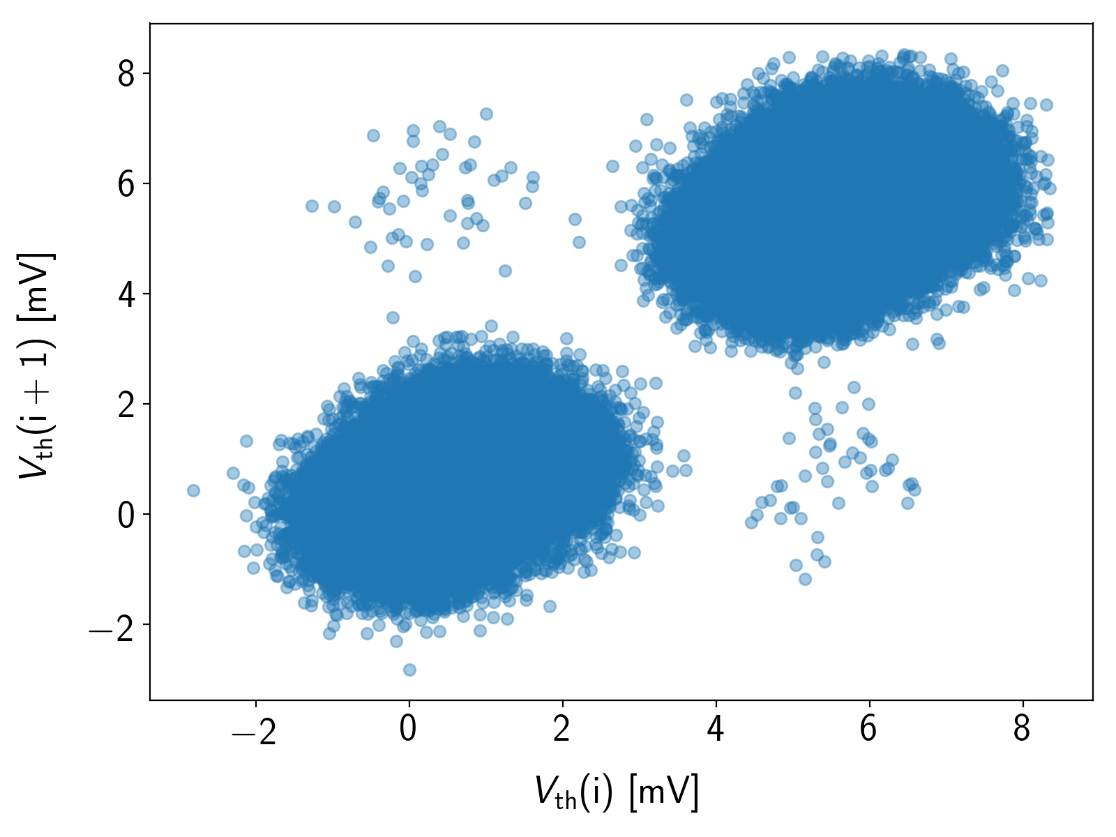
The lag plot method works by evaluating a correlation plot between neighboring measurement samples instead of binning them into a histogram (see Figure 6.8 and [133, 159]). The amplitude levels will then show up as clusters, one for each transition in the combined Markov chain of the system. The main benefit of this method is that also the transitions from one state to another can be observed as off-diagonal elements.

The time constants can be estimated by calculating the average duration time of being in a certain state (i.e. via the number of points in the clusters along the main diagonal). The calculation can be carried out in the same way as (6.37). On this occasion, it should be noted that the fraction of area $A$ and bin size $\mathrm {\Delta U}$ in (6.37) can be identified by the number of points attributed to the respective distribution. For the lag plot that means that when there is no overlap between the clusters, it is sufficient to simply count the points inside a certain cluster. The step heights can again be derived directly from the lag plot.

If the clusters are not separated well enough, clustering algorithms like the K-means algorithm and others can help to assign the individual points to a state. However, the benefits and drawbacks of certain algorithms and their application to RTN signals are beyond the scope of this work and can be found in [158, 161].

Although variations of this method were successfully used to extract the properties of multiple defects [162, 163], the main drawbacks of the lag plot method are its lacking robustness against measurement noise and its inability to detect thermal states.

6.6.3 Spectral Maps

The method presented here is heavily based on the spectral maps generated for the TDDS presented in Section 4.2.2 and [110, 116, 117, 164]. Its main benefit is that it uses step heights instead of absolute levels. This helps to mitigate both of the major problems of the methods explained in the previous sections. The spectral maps method has already been used successfully to obtain single defect properties from RTN signals in GaN/AlGaN fin-MIS-HEMTs [AGC5] and MoS2 FETs [AGJ7].

To construct the spectral maps, first of all a step detection algorithm which delivers the step times, the step heights and the sign of the steps is employed. A universal step detection algorithm should not be not influenced by long-term drift of the RTN signal. Linear filtering of the extracted step heights often also helps to filter some of the measurement noise from the extracted step heights.

Step Detection and Clustering

One of the most popular algorithms for edge detection, the Canny edge detection algorithm, is able to fulfill both of these requirements with a relatively low computational effort [165].

The variant of the algorithm used for step detection throughout this work is based on the convolution of the original signal $\dVth (t)$ with the derivative of a Gaussian distribution $g(t,\sigma _0)$ of width $\sigma _0$ .

$(6.38) \begin{equation} f(t) = \dVth (t) \ast \od {}{t} g(t,\sigma _0) \eqlabel {canny1} \end{equation}$

The resulting signal $f(t)$ is then free of long-term drift, with peaks for each sudden change in the signal (see middle picture in Figure 6.9). Further filtering is done by defining a threshold value for the signal $f(t)$ being $\pm n_\sigma \sigma _f$ with the standard deviation of the filtered signal $\sigma _f$ . A simple peak finding algorithm then selects the instance in time for all peaks above the threshold values. Thus the set of step times is

$(6.39) \begin{equation} t_\mathrm {s} = \mathrm {local\ max.}\lbrace |f(t)|>n_\sigma \sigma _f\rbrace . \eqlabel {canny2} \end{equation}$

Note that due to the linear Gauss filter, the step times will be shifted to the right by $\sigma _0$ . This can either be corrected manually, or the algorithm is applied for a second time with the time-inversed signal and the resulting step times are averaged. The step sizes for low-noise signals can simply be calculated by taking the values of the original signal before and after each step $t_{\mathrm {s},i}$ .

$(6.40) \begin{equation} \dVth {_{,i}} = \dVth (t_{\mathrm {s},i}+\Delta t) - \dVth (t_{\mathrm {s},i}-\Delta t) \eqlabel {canny3} \end{equation}$

For this naive approach to obtain (math image) , the noise in the extracted step heights is the same as the measurement noise. Thus, additional filtering of the step heights (i.e. mean or median filters, splines) potentially can be of advantage for very noisy signals. The results of the step-detection algorithm can be seen in Figure 6.9. In the upper picture, the original RTN signal is shown. In the middle picture of Figure 6.9, the resulting signal from (6.38) to extract the step times together with the applied threshold values can be seen. Finally, the lower picture gives the extracted steps after inserting the values from (6.39) into (6.40).

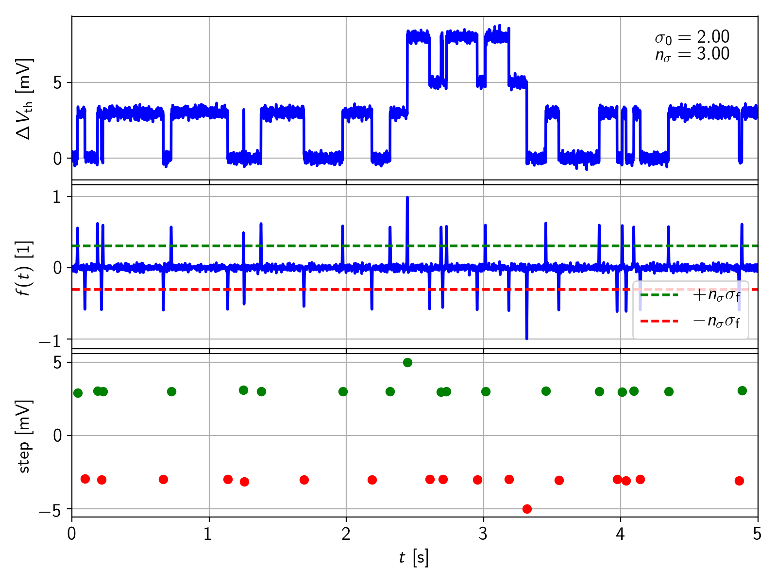
The free parameters $\sigma _0$ and $n_\sigma$ of the algorithm can be used to adjust the step detection to different signals:

• A larger value of $\sigma _0$ decreases the sensitivity to short-term peaks in the signal and thus helps to supress measurement noise. At the same time the sensitivity for fast defects decreases.
• A larger value of $n_0$ also helps to supress measurement noise but decreases the sensitivity for defects with small values of .

As the corresponding steps sizes of capture and emission events have opposite signs, the data from the detected steps then have to be clustered by the absolute value of the step sizes. Subsequently, the time differences between adjacent capture and emission events of each cluster are calculated. Any algorithm for the extraction of the times is highly dependent on the assumed Markov chain of the defect (more generally, the individual Markov chains of the defects for a system with multiple defects) and the accuracy of the step detection. Usually, some kind of state-machine is used to relate a certain capture event to a certain emission event and vice versa.

In this case, the steps are clustered with a K-means algorithm, developed independently by four different research groups [166–169]. The step data is divided into positive (electron capture) and negative (electron emission) events. Initial conditions for the algorithm are the assumed number of defects and the initial values of the assumed step heights, which then delivers the time sorted data to a simple state machine. Afterwards, the state machine calculates the time differences between two subsequent steps within one cluster if the two adjacent step directions possess different signs. Otherwise, if for example two positive steps occur after each other, the second one of the double-steps will be dropped. As this simple state machine does not allow two subsequent capture or emission events of the same defect, it is thus only suitable for extracting two-state defects.

Time Constants Extraction

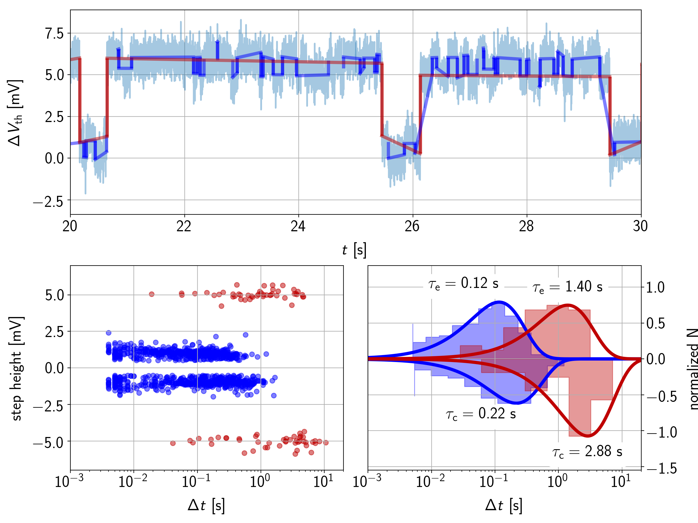
In Figure 6.10, the construction of the spectral maps and the subsequent extraction of the time constants is shown using the same two defects as in the previous sections. The upper picture shows parts of the RTN signal together with the results from the state machine. The discontinuities in the extracted signal are due to dropped double capture or emission events which emerge from inaccuracies in the step detection. The lower left picture gives the calculated time differences plotted into a spectral map. To obtain the characteristic times, an exponential distribution as given in (6.20) is fitted to each cluster. In the lower right picture, the extracted values, the histograms and the fitted distributions can be seen. The extracted time constants for the fast defect ( (math image) = 1 mV, = 0.1 s, = 0.2 s) and the slow defect (= 5 mV, = 2 s, = 3 s) in Figure 6.10 are both within 20 % error. This is actually a quite remarkable accuracy since both histograms suffer from opposite problems:

• The fast defect has many emissions and thus a good statistical foundation. The step detection is however very noisy due to the low value of , producing false-positives and missed steps in the clustering algorithm.
• The histograms of slow defect, on the other hand, contain quite few samples but very accurate clusters for capture and emission times.

In other words, errors due to inaccuracies in the step detection (and thus in the clustering) can be made up by a larger sample size while errors stemming from a small sample size can be made up by an accurate step detection.

Problems

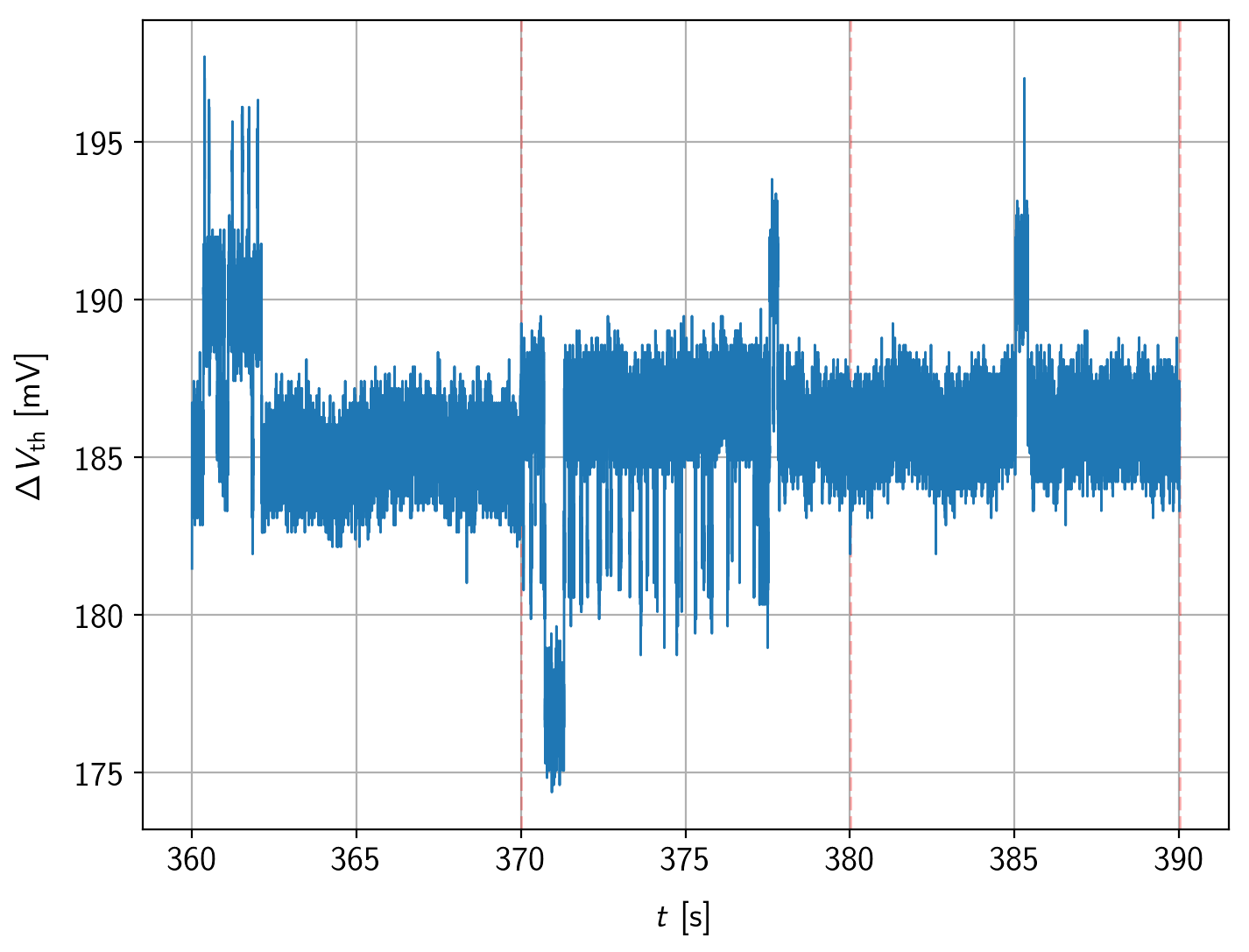
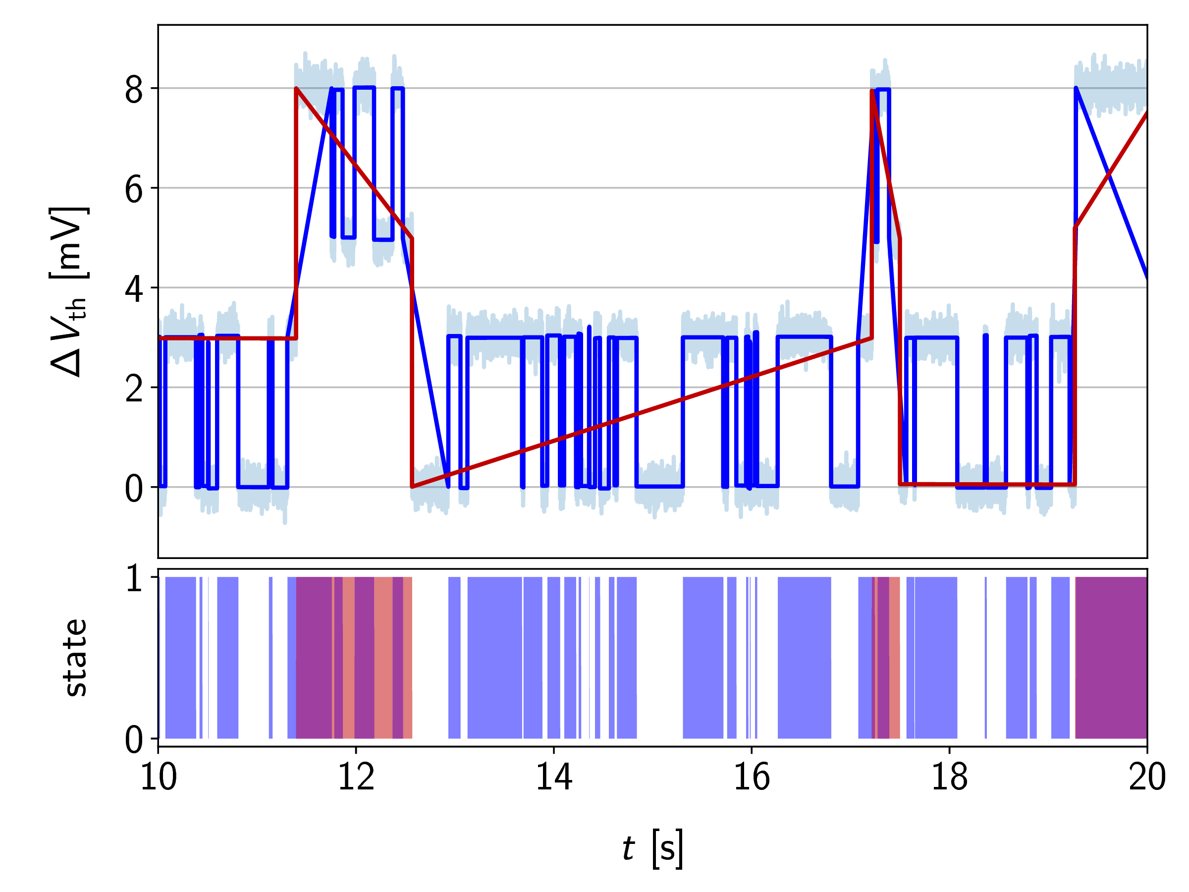
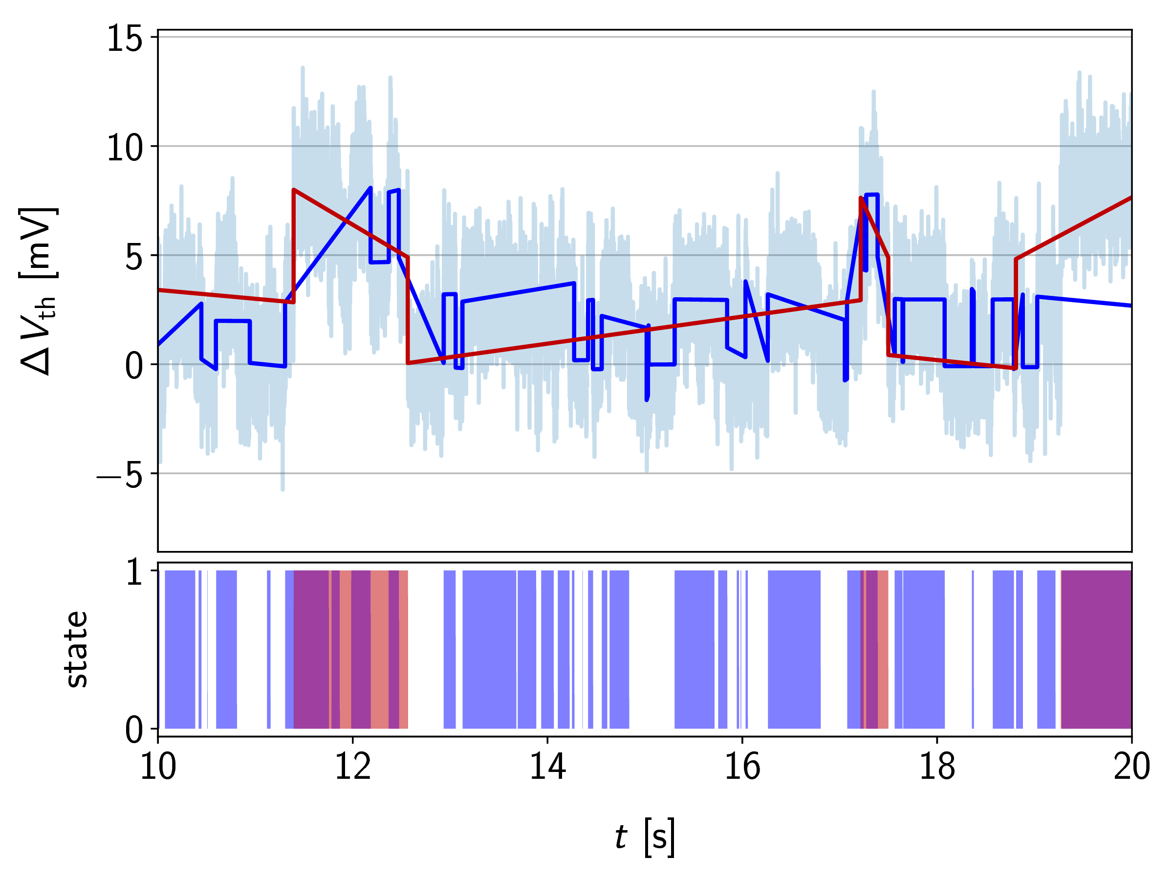
At a first glance, creating such state machines may look trivial, but for measurement data with a low SNR, multi-state defects as presented in Figure 6.4, or systems containing multiple defects with weakly separated step heights it can be prone to errors. As an example, we look at a simulation of two independent two-state defects with different levels of noise (see Figure 6.11). The step heights were set to 5 mV and 3 mV, the capture and emission times were 2 s/3 s for the 5 mV defect and 0.1 s/0.2 s for the 3 mV defect. The sampling rate was set to 1 kHz. After step detection, if the signal-noise ratio is sufficiently high, this allows to reliably extract the capture and emission times. On the other hand, if the signal quality is poor, errors in the step detection (i.e. missed steps or noisy step heights) will quickly degrade the accuracy of the extracted delta times.

Another problem with all of the methods presented in Sections 6.6.1 to 6.6.3 is that defects with thermal states (i.e. states with no charge transition) cannot be identified. A minor shortcoming of the spectral method is also that it is prone to errors if the bias regions with RTN activity from different defects with similar step heights overlap. This can be seen at the border regions of the two defect pairs (compare voltage regions in Figure 7.15). An example is shown in Figure 6.12, where signals of the overlapping regions from the defects investigated in Section 7.2 are plotted. A state machine for the extraction of the delta times as explained before will probably fail to map the observed emissions to the defects correctly. The impact of these falsely assigned emissions on the overall result highly depends on the cumulated number of capture and emission events. Thus defects with relatively slow time constants will be affected most.

Finally, the maximum time constants which can be extracted is practically limited by half of the recorded time of one measurement because at least one full transition on average is needed to calculate the time differences.

To be able to reliably quantify thermal states, multi-state defects and RTN produced by several different defects, a more robust method for the extraction of the characteristic time constants is needed. One method able to overcome most of the aforementioned shortcomings of the spectral method has been known for a long time in the context of machine learning and speech recognition. It is called the Baum-Welch algorithm which is able to train a HMM to a set of observations in a maximum-likelihood manner and will be explained in the next section.