Charge Trapping and Variability in CMOS Technologiesat Cryogenic Temperatures
3.2 2-State Nonradiative Multiphonon Model
The reason for the inaccurate bias and temperature dependence within the SRH model is that it ignores the structural reconfiguration at the defect site arising from changing charge states and the electrostatic shift of the trap level
due to the oxide field [174]. Since this deformation involves the emission/absorption of phonons, it is necessary to include the coupling to a surrounding phonon bath in the physical defect model to provide a physical
description of the whole system including all involved electrons and nuclei. Within first order perturbation theory, non-adiabatic transition rates in a system with both electrons and nuclei can be represented by their electronic and
vibrational wavefunctions  and
and  , respectively. The non-adiabatic charge transition rates can be obtained using Fermi’s golden rule

where the matrix element  is
is

Here,  and
and  represent a neutral and a charged state,
  and
and  are the corresponding vibrational eigenstate of and , respectively, with eigenenergies
  and
and  . The coupling operator
  describes the perturbation, while the Dirac delta distribution
  ensures energy conservation. The form of the vibrational wavefunctions depends on the Hamiltonian. Commonly a harmonic oscillation is used as a model Hamiltonian to describe the system as shown in Fig. 3.2. According to the Born-Oppenheimer approximation the electronic and vibrational wavefunctions can be treated separately, because the
nuclei are much heavier than the electrons and thus there is a large difference in their time scales of motion. Hence the electrons can always be assumed to be instantaneously in the ground state of the potential produced by the
positions of the nuclei, while the nuclei themselves move in an effective potential produced by the ground state electron distribution. Therefore, the Hamiltonian can be split in an electronic and a vibrational component
ensures energy conservation. The form of the vibrational wavefunctions depends on the Hamiltonian. Commonly a harmonic oscillation is used as a model Hamiltonian to describe the system as shown in Fig. 3.2. According to the Born-Oppenheimer approximation the electronic and vibrational wavefunctions can be treated separately, because the
nuclei are much heavier than the electrons and thus there is a large difference in their time scales of motion. Hence the electrons can always be assumed to be instantaneously in the ground state of the potential produced by the
positions of the nuclei, while the nuclei themselves move in an effective potential produced by the ground state electron distribution. Therefore, the Hamiltonian can be split in an electronic and a vibrational component

which allows to factorize the transition matrix element as follows

This final simplification is called Franck-Condon principle and  are referred to as Franck-Condon factors [175, 176, 177]. Using this simplification the transition rate (3.10) can be
represented by
are referred to as Franck-Condon factors [175, 176, 177]. Using this simplification the transition rate (3.10) can be
represented by

with the overlap integral

The electronic matrix element  describes the coupling between the respective electronic wavefunctions in the initial and final state, i.e. the coupling between the localized defect state and the delocalized valence/conduction band state of the charge
reservoir. The vibrational overlap
describes the coupling between the respective electronic wavefunctions in the initial and final state, i.e. the coupling between the localized defect state and the delocalized valence/conduction band state of the charge
reservoir. The vibrational overlap  is a measure for the nuclear tunneling probability. For a transition from one charge state to another all vibrational modes of the charge states must be taken into account. These vibrational modes can be described as a
canonical ensemble resulting in the total transition rate
is a measure for the nuclear tunneling probability. For a transition from one charge state to another all vibrational modes of the charge states must be taken into account. These vibrational modes can be described as a
canonical ensemble resulting in the total transition rate

where

is the weight of the excited initial vibrational wavefunction  and
and  is the partition function

This expression allows the definition of the lineshape function 

which contains all interactions of the vibrational states of the nuclei. The total transition rate (3.16) describes the transfer of a charge carrier between two electronic states. However, in a MOSFET device the states within the conduction and valence band of the semiconductor or in the metal gate form a continuum of states. To take all these states into account it is necessary ot integrate over all states of a band obtaining the rate equations

with  ,
,  being the density of states in the conduction and valence band, respectively, and
  ,
,  the Fermi-Dirac distribution for electrons and holes. Since in a semiconductor the charge carriers are located close to the conduction band edge
  and the valence band edge
  , it can be assumed that in a first order approximation the electronic coupling elements
  and the lineshape functions
  only depend on the band edges. This is called band edge approximation and allows to factor out
  and
and  from the integrals in (3.20).
The electronic coupling element  can be approximated by [174]

for electrons and holes, respectively, with  the thermal velocity,
  the capture cross section and
  being a tunneling factor, accounting for the spatial separation of the defect and the charge reservoir. The tunneling factor can be determined by solving the stationary Schrödinger equation. However, in most cases a
simplified WKB approximation is used to increase computational efficiency [178]. In the case of tunneling between the charge reservoir to the defect, the potentials can be approximated linearly. For computing the WKB
factor it is necessary to distinguish between direct tunneling and Fowler-Nordheim tunneling [179] depending on the shape of the potential barrier, as explained in more detail in [180].
being a tunneling factor, accounting for the spatial separation of the defect and the charge reservoir. The tunneling factor can be determined by solving the stationary Schrödinger equation. However, in most cases a
simplified WKB approximation is used to increase computational efficiency [178]. In the case of tunneling between the charge reservoir to the defect, the potentials can be approximated linearly. For computing the WKB
factor it is necessary to distinguish between direct tunneling and Fowler-Nordheim tunneling [179] depending on the shape of the potential barrier, as explained in more detail in [180].
An important parameter withing the entire model is the lineshape function that depends on the Frank-Condon factors and thus on the shape of the potentials of the defects. This potentials can be approximated as 1-dimensional [181, 182] harmonic, justified by the fact that in a Taylor expansion of the potentials the first order terms vanish and thus the second order term are dominant close to the equilibrium configuration [183]. Consequently, the potentials can be represented by harmonic potential energy curves (PECs) in the configuration coordinate (CC) diagrams, as can be seen in Fig. 3.2.

The PECs are described by the parabolic potentials

with  ,
,  being the vibrational frequency of the harmonic potential, which effectively describes the curvature of the parabola, and
  ,
,  being the corresponding masses. The analytical eigenfunctions of the harmonic oscillator are well known from literature and are given by

with  ,
,  being the Hermite polynomials, defined by
  . Using the analytic solutions for the vibrational states allows the computation of , however, this computation is expensive, even when using optimized algorithms which determine the vibrational overlap based on a recurrence relation as proposed by Schmidt [184]. Thus, in Section 3.2.1 a WKB-based approximation for the lineshape function is derived, which is computationally superior. However, at room
temperature and above the WKB-based approximation is not necessary, because the Frank-Condon factors, which are in essence the overlap of the vibrational wave functions of state and , are dominated by the overlaps close to the intersection point of the diabatic potentials
. Using the analytic solutions for the vibrational states allows the computation of , however, this computation is expensive, even when using optimized algorithms which determine the vibrational overlap based on a recurrence relation as proposed by Schmidt [184]. Thus, in Section 3.2.1 a WKB-based approximation for the lineshape function is derived, which is computationally superior. However, at room
temperature and above the WKB-based approximation is not necessary, because the Frank-Condon factors, which are in essence the overlap of the vibrational wave functions of state and , are dominated by the overlaps close to the intersection point of the diabatic potentials  and
and  [185]. Note that the intersection point can be computed analytically. For this, typically the following parameterization of the potentials is used

 is called relaxation energy and defined using the Huang-Rhys factor
  and is a measure for the electron-phonon coupling strength [186].
  and
and  are the curvatures of the harmonic potentials and define the curvature ratio
  while
while  describes the bias dependent energy difference of the minima of the two states, see Fig. 3.3.


With this parameterization the energy barrier is obtained as

which reduces to

for  . Note that in this classical description, the parameter
  becomes immaterial, since the lineshape function is only determined by the classical barrier height. Using this closed form expression for the intersection point of the potentials, the lineshape functions reduce to

with  . In the limit of high temperatures, the transition rates in (3.20) can then be simplified using the band edge
approximation [180] to
. In the limit of high temperatures, the transition rates in (3.20) can then be simplified using the band edge
approximation [180] to

This closed form allows a numerically fast computation of transition rates.
In this simplified classical approximation of the 2-state NMP model it is necessary to distinguish between strong electron-phonon coupling (SEPC) and weak electron-phonon coupling (WEPC), see Fig. 3.4. SEPC is the dominating mechanism for BTI degradation and describes charge transitions where the classical intersection point of the initial and the final potential energy surface lies between the two minima of the PECs. All other cases are subsumed as WEPC. For WEPC, which typically plays a minor role for BTI degradation [180], classical barriers are given as shown in Table 3.1.

Figure 3.4: Depending on trap parameters and applied gate voltage, the charge transition takes place in the strong (left) or in the weak (right) electron-phonon coupling regime. In the SEPC regime, the classical intersection lies in between the minima of the two PECs, while in the WEPC regime it lies outside of the minima.


This derived classical approximation for the 2-state NMP model works well for room temperature and above, however, in the limit of low temperatures the simplified lineshape functions (3.27) would freeze out completely

and there would be no charge trapping in cryogenic environments. However, measurements show that there are still electrically active traps at cryogenic temperatures, as will be discussed in detail in Part II of this work. The reason for this is that at low temperatures the assumption that the overlaps of the vibrational wavefunctions close to the intersection points of the diabatic potentials dominate does not hold anymore, because those states cannot be excited anymore at low temperatures. Thus, vibrational states at lower energies dominate the overlap and hence the lineshape function. This makes it necessary to include all vibrational states in the computation of the transition rate.
3.2.1 WKB Approximation
The computation of the full quantum mechanical charge transition rate (3.19) is inefficient and thus not suitable for calculating the defect model within device or circuit simulation tools. However, the classical approximation breaks down at cryogenic temperatures and can thus also not be used. Therefore, an approximation based on the Wentzel–Kramers–Brillouin (WKB) method combined with the saddlepoint method was proposed by Holstein [187] and further developed by Markvart [188, 189, 190]. These approximations where developed for the weak electron-phonon coupling regime, however, for charge trapping most transitions happen within the strong electron-phonon coupling regime. To make this method suitable for reliability studies of MOS devices a more generalized form of the approach is developed. In the following the approximation of the full quantum mechanical lineshape function is based on the idea that the vibrational wavefunctions can be approximated by a WKB-based terms. This approximation allows switching from a summation over the exact discrete eigenenergies to a continuous integral form. The integrals can be evaluated using the saddlepoint method. This allows finding an effective barrier which is lower than the classical barrier and thus prevents the transition rates from freezing out. The full derivation is given in the following.
For deriving a general formulation for the WKB approximation a transition  is singled out by introducing

with the vibrational overlap integral given by

By approximating the PECs as harmonic, the vibrational wave functions can be expressed analytically by (3.23). The parabolic PECs for a charged and a neutral configuration are shown in Fig. 3.5, together with their eigenfunctions, and the vibrational wavefunctions which are shown with dashed lines. While this analytical expression is suitable for the lower eigenfunctions, the Hermite polynomials becomes very large for higher energy levels leading to numerical instabilities.

Figure 3.5: The vibrational wavefunctions of harmonic potential energy surfaces can be computed analytical. Since the analytical expressed wavefunctions (dashed lines) are rather complicated and unwieldy for simplifications, a WKB approximation (solid lines) is used which describes the wavefunctions in the classically forbidden regions well by capturing the exponential decay.
For solving the integration in (3.31) efficiently, a WKB-based approximation of the wavefunction  introduced in (3.23) is used. The idea of the WKB approximation is a semi-classical series expansion of a corresponding action
with respect to
introduced in (3.23) is used. The idea of the WKB approximation is a semi-classical series expansion of a corresponding action
with respect to  . In principle, this expansion could be carried out at any point, however, typically it is done at the classical turning point
  . This case is also shown in Fig. 3.5. The expansion can be classified in three regions, a classically allowed region between the
turning points and
. This case is also shown in Fig. 3.5. The expansion can be classified in three regions, a classically allowed region between the
turning points and  , which is described by an oscillating function and the classically inaccessible regions which can be described by exponentially decaying functions (solid lines). The oscillating function cancels out approximately when
integrated and thus can be neglected [190]. In a similar manner, the exponentially decaying function which is far away from the classical intersection point can be neglected. Therefore, the WKB wavefunction reduces to a single
exponentially decaying function in the classically prohibited region
, which is described by an oscillating function and the classically inaccessible regions which can be described by exponentially decaying functions (solid lines). The oscillating function cancels out approximately when
integrated and thus can be neglected [190]. In a similar manner, the exponentially decaying function which is far away from the classical intersection point can be neglected. Therefore, the WKB wavefunction reduces to a single
exponentially decaying function in the classically prohibited region

with  being the classical momentum. The full derivation of the WKB method is given in Appendix A.1. By normalizing
  the constant
  can be computed, with being the oscillator frequency [190]. The idea can also be seen in Fig. 3.5: The dashed lines show the analytical vibrational
functions (3.23), while the solid line is divided in the three regions, two exponential decaying and a oscillating region. The integration is only
done in the shaded regions below the classical intersection point, since all other terms cancel out approximately. Close to the classical turning points a singularity can be seen. Such singularities occur due to the Taylor expansion
used for the WKB approximation, as explained in Appendix A.1. However, the overlap is dominated far away from the singularity, thus the singularity gets neglected in the
integration when using the saddlepoint method, as explained in detail later in this section. For the calculation of the exact LSF given in (3.19),
one does not have to explicitly distinguish between weak and strong electron-phonon coupling, hence the calculation is always the same regardless of the relative positions of the PEC. However, by reduction to the exponential
decaying functions in the classically prohibited region, the sign of the decaying part needs to be considered. In the following, the deviation is done for the strong-electron-phonon coupling case, all occurring cases are shown in
Fig. 3.6 and are considered in the sign of the final result.
can be computed, with being the oscillator frequency [190]. The idea can also be seen in Fig. 3.5: The dashed lines show the analytical vibrational
functions (3.23), while the solid line is divided in the three regions, two exponential decaying and a oscillating region. The integration is only
done in the shaded regions below the classical intersection point, since all other terms cancel out approximately. Close to the classical turning points a singularity can be seen. Such singularities occur due to the Taylor expansion
used for the WKB approximation, as explained in Appendix A.1. However, the overlap is dominated far away from the singularity, thus the singularity gets neglected in the
integration when using the saddlepoint method, as explained in detail later in this section. For the calculation of the exact LSF given in (3.19),
one does not have to explicitly distinguish between weak and strong electron-phonon coupling, hence the calculation is always the same regardless of the relative positions of the PEC. However, by reduction to the exponential
decaying functions in the classically prohibited region, the sign of the decaying part needs to be considered. In the following, the deviation is done for the strong-electron-phonon coupling case, all occurring cases are shown in
Fig. 3.6 and are considered in the sign of the final result.

Figure 3.6: There are 8 different relative positions of the potential energy surfaces which need to be considered in the WKB based approximation of the transition rate: 4 positions in the weak electron-phonon coupling regime
and 4 in the strong coupling regime. Furthermore, it is necessary to consider if the initial state is energetically above or below the final state and if the classical barrier  is above or below the ground state
  .
.
As previously mentioned, the overlap integral (3.31) can be simplified using the saddlepoint method [191]. For this, the overlap integral is first simplified using the WKB wavefunction (3.32) to get

where the phase  is given by

Exploiting the fact that the integral is dominated by the region near the point of stationary phase, which is given by  , which can be verified by solving for
  , the integral can be expressed as a function of only:

For this, the saddlepoint method is used, which is derived in Appendix A.2 and allows the simplification of a general integral  of the form

when  and
and  hold. Note that the overlap integral is not exactly of this form, due to the
  dependence of the non-exponential prefactor. However, this can be neglected, since the integral is dominated by the exponential term. A further simplification requires to convert the quantized lineshape function
containing and to a continuous form
dependence of the non-exponential prefactor. However, this can be neglected, since the integral is dominated by the exponential term. A further simplification requires to convert the quantized lineshape function
containing and to a continuous form

by using ![\( E_{i\alpha }\xrightarrow []{}E \)](draftv0-images/CDC379B030B8282343EF98BC8E8F0E2B.svg) and
and ![\( E_{j\beta }\xrightarrow []{}E’ \)](draftv0-images/67B7DBA32E41F4B04FB55597B1E1EDE6.svg) . The same can be done for the summation of the eigenenergies
. The same can be done for the summation of the eigenenergies
![(3.38) \{begin}{align} \sum \limits _{\alpha =0}^\infty f(E_{\alpha }) \xrightarrow []{} \int \limits _{E_0}^\infty f(E) \frac {\mathrm {d}n\alpha }{\mathrm {d}E}\mathrm {d}E.
\{end}{align}](draftv0-images/image-268.svg)
Here,  is the density of states of the quantum mechanical harmonic oscillator

The continuous lineshape function (3.37) can be used to express equation (3.19) as

Evaluating the Dirac delta distribution and using the simplified version of the overlap integral (3.35), the rate equation (3.40) simplifies to

with  being the continuous form of
  . The term
  contains all non-exponential terms depending on

By applying the saddlepoint method a second time, the integral (3.41) can be evaluated at the extremum 

leading to

After insertion of all terms the final result reads

For obtaining the occurring phase  in the final result it is necessary to compute the integral (3.34). This can be done analytically, resulting in the expression

From this expression it is possible to get an analytic expression for the second derivative  and
and  . The factors
  ,
,  ,
,  and
and  are necessary to differentiate between WEPC and SEPC. Furthermore it is necessary to differentiate between an initial state having a higher or a lower energy level than the final state and if the classical intersection point
is above or below the ground state of the initial or final state. The different occurring cases are shown in Fig. 3.6 and the signs for the
different cases are listed in Tab. 3.2.
are necessary to differentiate between WEPC and SEPC. Furthermore it is necessary to differentiate between an initial state having a higher or a lower energy level than the final state and if the classical intersection point
is above or below the ground state of the initial or final state. The different occurring cases are shown in Fig. 3.6 and the signs for the
different cases are listed in Tab. 3.2.
|
|
|
|
|
 |
1 | -1 | -1 | -1 |
 |
1 | 1 | 1 | -1 |
 |
-1 | 1 | 1 | 1 |
Table 3.2: Factors in analytic expression (3.46) of the overlap integral
3.2.2 Benchmark of the WKB-Based 2-State NPM Approximation
The derived WKB-based approximation of the 2-state model is developed for the limit of low temperatures. However, since characterization is often done in a broad temperature window (in this work specially from room temperature to 4 K) it is important to define the limits of the approximation and to check carefully if the models remain valid over the whole characterization range.
Lifetime Broadening
For benchmarking the WKB based approximation against the full quantum mechanical model it is necessary to introduce a lifetime broadening of the Dirac delta distribution  occurring in the lineshape function (3.19) [192]. Without this broadening, the overlaps of the wave functions would
only be nonzero for perfect energy level alignment
occurring in the lineshape function (3.19) [192]. Without this broadening, the overlaps of the wave functions would
only be nonzero for perfect energy level alignment  . Therefore, the Dirac delta distribution is replaced by a Gaussian distribution

with  being the width of the broadening. The choice of is crucial, however, not trivial. Since the broadening is a thermal effect, should show a temperature dependence, thus the simplest form of a linear dependence
  was chosen. At cryogenic temperatures this broadening would disappear, however, excited states still show a finite lifetime due to phonon emissions, and thus must be somehow affected by lifetime broadening. Therefor,
a sigma of the form
was chosen. At cryogenic temperatures this broadening would disappear, however, excited states still show a finite lifetime due to phonon emissions, and thus must be somehow affected by lifetime broadening. Therefor,
a sigma of the form

was chosen, where  is a constant normalized to the level energy spacing
  which has the role of representing temperature independent lifetime broadening due to phonon emissions. A variation of this constant is shown in Fig. 3.7 for between 1/5 and 3. Different values for lead to different saturation values of the lineshape function towards cryogenic temperatures. The impact of gets smaller in the classical limit where the lineshape functions approach the classical model for all chosen . As can be seen, shows a saturation towards smaller values. The difference between
  and
and  is quite small compared to the larger values. In this work
  was chosen, to guarantee that there is always at least one overlap of vibrational functions in the range of
  .
.

Figure 3.7: The benchmarking of the WKB based approximation against the full quantum mechanical model makes it necessary to smear out the Dirac delta distribution in the lineshape function (3.19) to a Gaussian function. The impact of different smearing widths can be seen for different
minimal widths between  and
and  .
.
Temperature Dependence
The main motivation for using the full quantum mechanical model or the WKB based approximation in favor of the much simpler classical approximation is to ensure the validity of the computed transition rates at cryogenic temperatures. Therefore, the benchmarking of the WKB based approximation against the full quantum mechanical model is specially relevant for temperatures below room temperature.

Figure 3.8: The full quantum mechanical lineshape function (solid) and the WKB based approximation (dashed) for ,  and
and  do not freeze out for different configuration coordinate displacements
  , while the independent classical approximation (dotted) freezes out completely towards 4 K (left). This can be mapped to an effective barrier lowering, which shows that the effective barrier is 0 eV at cryogenic
temperatures, while the classical effective barrier is almost temperature independent (right).
, while the independent classical approximation (dotted) freezes out completely towards 4 K (left). This can be mapped to an effective barrier lowering, which shows that the effective barrier is 0 eV at cryogenic
temperatures, while the classical effective barrier is almost temperature independent (right).
The lineshape function can be seen for a variation of temperatures between 4 K and 500 K in Fig. 3.8 for different
configuration coordinate displacements between  and
and  . The full quantum mechanical model (solid) and the WKB based approximation are almost perfectly on top of each other. Depending on the displacement the lineshape function starts to get constant below a certain temperature, while the classical approximation of the lineshape function, shown as black dotted line, is independent and freezes out completely towards cryogenic temperatures. Using the computed lineshape function, it is possible to plot the effective barrier

which can be derived directly from the Arrhenius law [185]. The effective barrier decreases to 0 eV at low temperatures as can be seen in Fig. 3.8 (right). Towards high temperatures the effective barrier approaches the classical barrier. However, at room temperature there is
still a significant difference between the classical barrier and the effective barrier for small , which means that the classical approximation underestimates charge transition rates of defects with small configuration coordinate displacements by neglecting nuclear tunneling. The classical barrier shows only a small
temperature dependence arising from the temperature dependent prefactor in the classical lineshape function.
The lineshape function can be seen for a variation of the energetic displacements in Fig. 3.9. For low temperatures, the classical lineshape function gives reasonable values only in a very small displacement window, in which the classical barrier is close to 0 eV. The full quantum mechanical lineshape function and the WKB based approximation on the other hand give comparable large values over a wide range of energetic offsets, which explains the observed freeze-out of transition rates in the classical approximation.
.svg)
Figure 3.9: The forward and reverse lineshape functions  and
and  at
at  (blue),
  (violet),
  (magenta) and
  (red) for different energetic displacements show that the classical approximation (dotted) gives large values only in a very narrow interval where the classical barrier is close to 0 eV, while the full quantum mechanical version (solid) and the WKB based
approximation (dashed) have large values for a comparable wide interval.
(red) for different energetic displacements show that the classical approximation (dotted) gives large values only in a very narrow interval where the classical barrier is close to 0 eV, while the full quantum mechanical version (solid) and the WKB based
approximation (dashed) have large values for a comparable wide interval.
Parameter Scan
For a systematic comparison of the WKB based approximation and the full quantum mechanical lineshape function the parameters  , , , , and
  are being varied. The variation of these parameters is done using the grid given in Tab. 3.3
| Parameter space | |||
| Parameter | min. | max. | gridpoints |
| [eV] |
0.5 | 6 | 10 |
 [eV] [eV] |
-3 | 3 | 10 |
[ ] ] |
1 | 6 | 10 |
| [1] |
0.7 | 1.3 | 3 |
| T [K] | 4 | 500 | 10 |
Table 3.3: For benchmarking the WKB-based approximation against the full quantum mechanical transition rate of the 2-state NMP model the parameters defining the potential energy curves, and thus the transition rates, are varied in the parameter space given above.
The lineshape function is computed for every combination of grid point parameters. Since the lineshape function varies over many orders of magnitude, the logarithmic lineshape function is used for defining the relative error made by the WKB-based approximation compared to the full quantum mechanical computation

For the parameter variation shown in Tab. 3.3 more than  of the parameter combinations result in a
  in the interval
 ![\( [-1,1] \)](draftv0-images/0EF7964444753B15CF70018E82A764B4.svg) , which corresponds to a difference of less than one order of magnitude (for a quantity which varies over tens of orders of magnitudes). This is illustrated in Fig. 3.10. Note that larger differences between the WKB-based approximations and the full quantum mechanical 2-state model arise
for temperatures above 300 K. Here the overlap integral is not dominated by the exponential tail and therefore the WKB-approximation leads to larger deviations.
, which corresponds to a difference of less than one order of magnitude (for a quantity which varies over tens of orders of magnitudes). This is illustrated in Fig. 3.10. Note that larger differences between the WKB-based approximations and the full quantum mechanical 2-state model arise
for temperatures above 300 K. Here the overlap integral is not dominated by the exponential tail and therefore the WKB-approximation leads to larger deviations.

Figure 3.10: More than of the parameters listed in 3.3 result in a relative error of the logarithmic lineshape function in the interval . This corresponds to a difference of one order of magnitude which is considered acceptable in the context of transition rates which typically vary over many decades.
Computational Costs
As shown in the previous section, the WKB based approximation gives very accurate results for the lineshape function over many orders of magnitude and a wide range of parameters. Here the focus is set on analyzing the
computational performance of the WKB approximation, which is important in the context of compact modeling. The computation time of the full quantum mechanical model depends on the number of vibrational states which
need to be considered, see Fig. 3.11. Large relaxation energies and large energetic offsets lead to a higher number of vibrational states contributing to the lineshape function. Thus, with an increasing the number of not negligible elements in the overlap matrix grows, scaling with  where
where  is the index of the highest included vibrational state. Since the computation of the overlap matrix is the bottleneck of the full quantum mechanical model, the overall runtime of the exact model also scales with , as is clearly shown in Fig. 3.11. The bottleneck of the WKB based approximation is to minimize (3.43) for finding
  . Finding can be done by using e.g. Newton’s method or other root-finding algorithm. Here, the energetic offset has no impact on the root-finding algorithm as can be seen in the Fig. 3.11.

Figure 3.11: The number of vibrational states contributing to the lineshape function increases with increasing and with it the number of elements in the overlap matrix (black line). Since the computation of the overlap matrix is the bottleneck of the full QM lineshape function (blue), the computation time increases with the same
slope as the elements in the overlap matrix. The numerical bottleneck of the WKB bases model (red) is finding the energy , which is independent of the number of vibrational functions.
With this numerical advantage of the WKB based model over the full quantum mechanical 2-state NMP model defect sampling of thousands of defects is possible. However, the WKB based model is not a closed form expression in
the form of an equation set, because a root-finding algorithm needs to be applied for finding the effective energy . By assuming that the PECs of the two states have identical curvatures, the WKB-based approximation can be further simplified to a real closed form expression, as discussed in the next section.
3.2.3 Approximation for Undistorted Potential Energy Curves
The WKB-based approximation for the 2-state NMP model is very accurate and numerically superior to the full quantum mechanical summation. However, since finding the effective barrier in the WKB-based approximation requires a Newton solver, it is not a closed form solution and is thus numerically expensive compared to the classical approximation. To further improve the computational performance,
the number of free parameters in the defect sampling can be reduced by assuming that the deformation of PECs during charge trapping can be neglected, which is done by fixing the curvature ratio of the PECs to  . This is a reasonable approximation and known from the classical model since
  and are correlated in the 2-state NMP model, allowing to fix by adapting . By developing a Taylor expansion of the classical barrier
  with respect to the energetic offset
  [MJJ2]

it can be seen that for a wide range of values a corresponding can be found resulting in the same , see Fig. 3.12. This allows finding  pairs which are experimentally almost indistinguishable. While in previous studies large curvature ratios like
  [136] have been used, this correlation allows using smaller ratios in the value range of
  , which is the typical range for oxide defects as extracted from DFT calculations [MJJ2, 185].
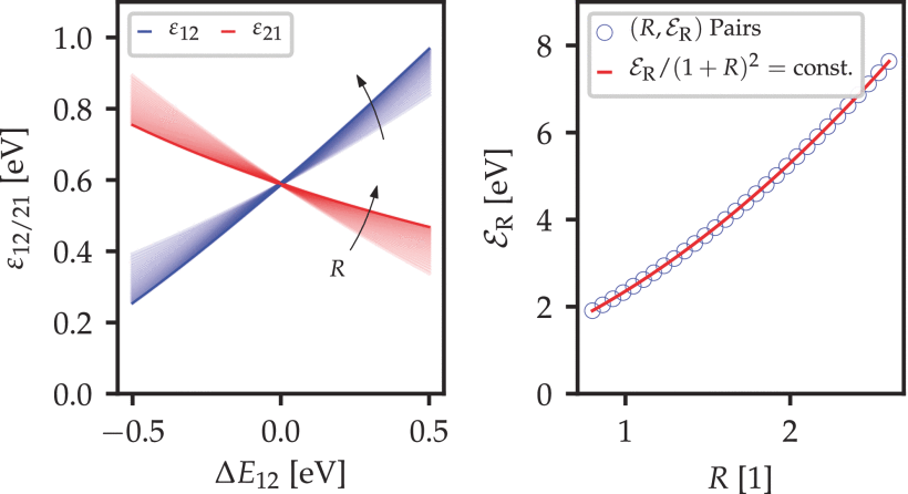
Figure 3.12: The charge transition barriers  are experimentally very similar for a large set of
  pairs along the curve
  This can be derived using a Taylor expansion of the classical transition barrier (3.51) and allows to fix either or .
By fixing , the WKB-based approximation can then be considerably simplified [193]. The lineshape function  can be computed by

with

and the dominant mode  where
where

and

The oscillation frequency  can be calculated directly from the relaxation energy for a given configuration coordinate offset

Since ,  holds and is referred to as . The energy levels
  and
and  in (3.52) are given by

This set of equations allows a direct computation of the transition rate in the strong electron-phonon coupling for the case that the final state is lower than the initial state. The backward rate (which can not be computed with this set of equations, because here the final state would be energetically higher than the initial state) can be computed directly from detailed balance as it is done in classical 2-state NMP theory [180]. For the case of weak electron-phonon coupling, the effective barrier can be replaced by the fixed values derived in [136, 180].
The lineshape function can also be used for computing the effective barrier  by
by

The closed form expression for the lineshape function for undistorted potential energy curves matches well with the full quantum mechanical 2-state model as can be seen in Fig. 3.13 for  and
and  for various configuration coordinate offsets.
_R=1.svg)