Charge Trapping and Variability in CMOS Technologiesat Cryogenic Temperatures
7.3 Random Telegraph Noise
On small area devices single charge capture and emission events are observed in the measured drain-source current or the corresponding  curve as discrete steps. Every defect can therefore be identified by
  , where
  is the mean step height (either in the current or the equivalent
  representation) and
  and
and  are the mean capture and emission times, respectively. This set of parameters can be found for various gate voltage and temperature conditions
  . It has to be noted that the step heights and the charge transition times are stochastic quantities. The step height is normally distributed around a mean value. As the charge transition times can be described as a Markov
process, it can be shown using the Master equation that capture and emission times are exponentially distributed [174], as can be seen for the exemplary trace in Fig. 7.3.
. It has to be noted that the step heights and the charge transition times are stochastic quantities. The step height is normally distributed around a mean value. As the charge transition times can be described as a Markov
process, it can be shown using the Master equation that capture and emission times are exponentially distributed [174], as can be seen for the exemplary trace in Fig. 7.3.
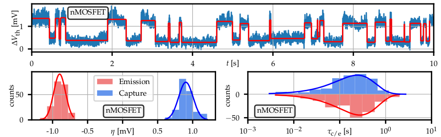
Figure 7.3: After detecting the steps of an arbitrary RTN signal (top) various parameters such as the step heights or charge capture and emission times can be extracted. Based on this it can be seen that step heights of capture and emission are normally distributed around the same absolute value. Capture and emission times are exponentially distributed shown here using a logarithmic x-axis.
For the extraction of the distributions of step heights, time constants and the corresponding set of mean parameters which identifies a defect, a precise detection of the position of the discrete steps is crucial. Since there should be ideally tens or hundreds of discrete steps in a single RTN trace, and typically multiple traces for different
temperatures and gate voltage conditions are needed, an automatic or semi-automatic detection algorithm of the position and heights of the steps is required. In this work, two different algorithms were used: the Canny edge
detector and Otsu’s method which will be presented in the following sections.
7.3.1 Canny Edge Detector
The Canny edge detector was developed by John F. Canny in 1986 and was initially designed to detect edges in images [235]. While the original algorithm was developed for 2-dimensional applications, the step detection in RTN signals is a 1-dimensional problem which simplifies the algorithm considerably. Analogous to the deviation in [140], the algorithm can be broken down into the following steps, shown in Fig. 7.4:
-
1. The intensity of the measured RTN signal
 increases when convoluting it with a discretized first derivative of a Gaussian filter
where
 is the width of the truncation and
with
 being the width of the Gaussian filter.
-
2. The convuluted signal
![\( R[n] \)](draftv0-images/A290488BCEAF580036E2F3E8A0DDDCE4.svg) can be simplified by applying a non-maximum suppression
can be simplified by applying a non-maximum suppression
-
3. A threshold value
 is chosen, which suppresses responses from noise:
![(7.9) \{begin}{align} R[n] = (S*G)[n]\sum \limits _{k=-W}^W S[k]G’[n-k], \{end}{align}](draftv0-images/image-923.svg)
![(7.10) \{begin}{align} G’[t] = -\frac {t}{\sqrt {2\pi }\sigma ^3}\mathrm {e}^{-\frac {t^2}{2\sigma ^2}} \{end}{align}](draftv0-images/image-925.svg)
![(7.11) \{begin}{align} R_\mathrm {m}[n] = \left \{\begin {array}{ll} R[n], & (|R[n]|>R[n+1] \wedge |R[n]|>R[n-1]) \\ 0, & \mathrm {else}\end {array}\right . .
\{end}{align}](draftv0-images/image-928.svg)
![(7.12) \{begin}{align} R_\mathrm {t}[n] = \left \{\begin {array}{ll} R[n], & (|R_m[n]|>R_\mathrm {th}) \\ 0, & \mathrm {else}\end {array}\right . . \{end}{align}](draftv0-images/image-930.svg)

Figure 7.4: The Canny edge detector can be broken down into the following steps: An initial RTN signal (top panel) is folded with the derivative of a Gaussian filter  . The resulting signal
  (central panel) shows distinctive peaks. The signal is simplified by a non-maximum suppression before setting a threshold value (red/green). Peaks with an absolute value above the threshold are detected as steps (bottom panel), the sign of the step allows to differ between
up-steps and down-steps which correspond to charge capture and emission events.
(central panel) shows distinctive peaks. The signal is simplified by a non-maximum suppression before setting a threshold value (red/green). Peaks with an absolute value above the threshold are detected as steps (bottom panel), the sign of the step allows to differ between
up-steps and down-steps which correspond to charge capture and emission events.
The sign of ![\( R_\mathrm {t}[n] \)](draftv0-images/A17F7B1D9E580B3A5DAF74BB0D43A3CB.svg) determines whether an upwards or downwards step is detected, and the height of the step can be extracted from the original signal. This algorithm has a low error rate and the localization of the edges is very precise. If
there are two active defects in a single signal, the detected steps can be clustered by their step heights using for example a K-means algorithm [236]. However, the algorithm has the disadvantage that the width of the
Gaussian filter and the threshold value are input parameters which have be to varied to detect different active defects. Thus the detection quality depends on the selected parameters. However, when dealing with a large set of RTN signals, a fully automated
algorithm for step detection is necessary, like for example Otsu’s method which is presented in the next section.
determines whether an upwards or downwards step is detected, and the height of the step can be extracted from the original signal. This algorithm has a low error rate and the localization of the edges is very precise. If
there are two active defects in a single signal, the detected steps can be clustered by their step heights using for example a K-means algorithm [236]. However, the algorithm has the disadvantage that the width of the
Gaussian filter and the threshold value are input parameters which have be to varied to detect different active defects. Thus the detection quality depends on the selected parameters. However, when dealing with a large set of RTN signals, a fully automated
algorithm for step detection is necessary, like for example Otsu’s method which is presented in the next section.
7.3.2 Otsu’s Method
Otsu’s method is an algorithm for automatic thresholding and was developed by Nobuyuki Otsu in 1979 [237]. Just like the Canny edge detector, Otsu’s method was initially designed for image thresholding, thus for
separating pixels into two classes: foreground and background. The algorithm searches for a threshold value which maximizes the inter-class variance of the two classes  and
and  equivalent to minimizing the inter-class variance. This process is performed in four steps:
-
1. The normalized histogram and the probability
 for every bin
  of
of  bins in total is computed. The normalized histogram for the signal in Fig. 7.5 (left) can be seen in Fig. 7.5 (right).
-
2. The class probabilities
 and class means
  are initialized for
  .
.
-
3. Next, the algorithm steps through all thresholds
 and computes the class probabilities
  , the class means
  and the inter-class variances
  . Here, the class probabilities are defined as
Using the class probabilities, the class means
are obtain as
which allows to compute the inter-class variance
In Fig. 7.5 (right) the inter-class variance is plotted for every threshold value.
-
4. Finally, the optimum threshold value is determined as the threshold
 for which the respective inter-class variance is maximized.


![(7.15) \{begin}{align} \sigma _b^2(t) = \omega _0(t)\omega _1(t)[\mu _0(t)-\mu _1(t)]^2. \{end}{align}](draftv0-images/image-953.svg)
After obtaining the threshold with Otsu’s method, a step in the signal at timestep is given at those points, where

holds.

Figure 7.5: For a RTN signal (left) a normalized histogram (right) with bins is computed. For every bin, the inter-class variance  can be calculated and the bin with the maximum gives the best threshold value. The positions where the signal switches from above to below the threshold value can be extracted and corresponding step heights and time constants are obtained.
Compared to the Canny edge detector, Otsu’s method has the advantage that the thresholding is completely automated. In general, it can be beneficial to apply a filter before the automated thresholding to suppress measurement noise. While this has the disadvantage that very short time constants get lost, it renders the thresholding extremely robust and even allows the detection of small step heights. In this work, the denoising algorithm proposed by Chambolle was used [238].
Otsu’s method can only be applied on measurement data including a single active defect. In case of the detection of multiple active defects (multi-level RTN) typically only the most prominent defect signal will be extracted. To avoid incorrect detection additional sanity checks are applied, e.g. a Kolmogorov-Smirnov test for testing if capture and emission times follow an exponential distribution. For a detailed analysis of multi-level RTN more advanced techniques as a factorial hidden Markov model analysis are needed [239].