The standard Knudsen diffusion calculation discussed in Section 3.2 requires substantial approximations. Namely, the sticking coefficients are assumed to be low, and the features
are assumed to be long, such that the diffusion process can be approximated by the diffusivity of infinite cylinders or trenches. Therefore, local contributions to the flux due to visibility of the source (c.f. Section 2.3.2) are neglected. Although Clausing has calculated corrections in transmission probabilities for short cylinders [114, 115], the issue of direct source flux contributions remains
unaddressed.
The hitherto discussed formulation of Knudsen diffusivity including the view factors enables an extended calculation overcoming these limitations for short cylinders and including the direct flux in a straightforward manner. In
essence, the mass balance procedure follows the same derivation that Eq. (3.15), however, the preferential transport direction
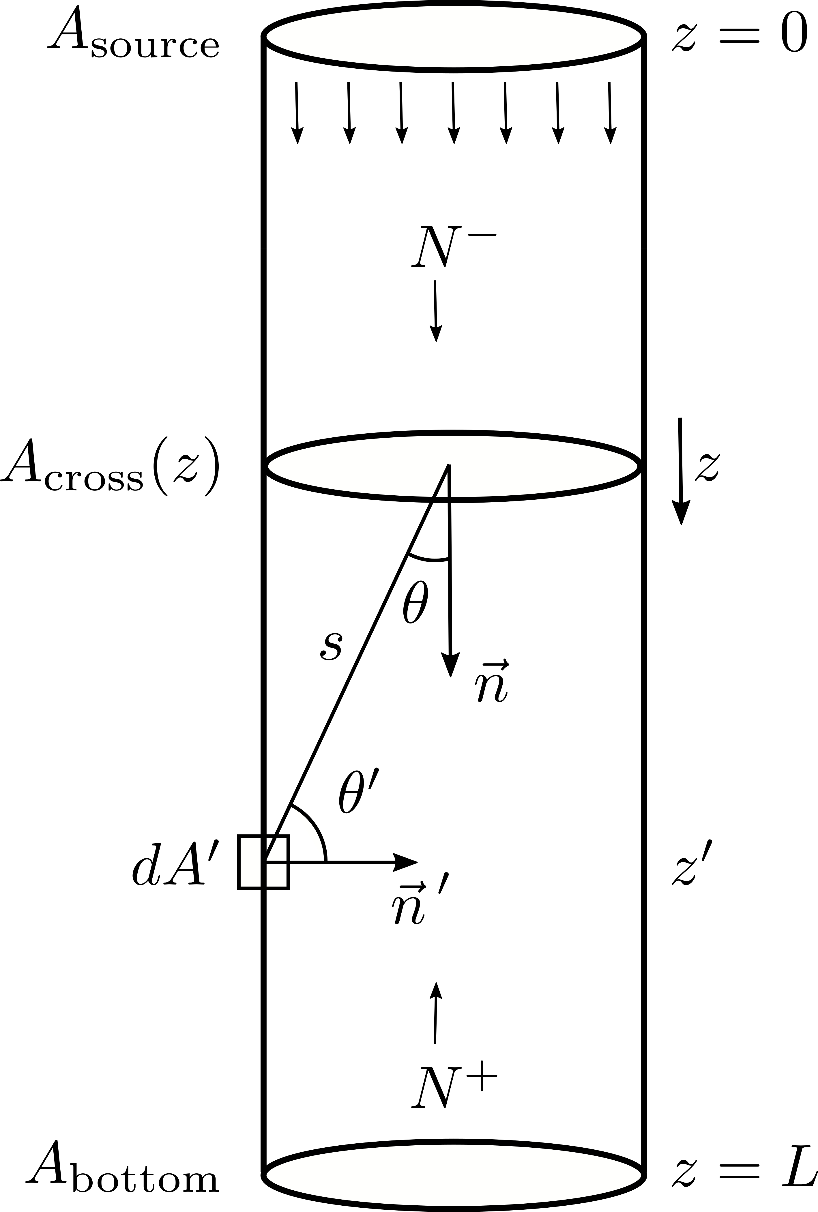
\(z\) is no longer assumed to extend from \(-\infty \) to \(\infty \). Instead, the same mass balance integrals to calculate \(\Gamma _\mathrm {cross}\) from Eq. (3.12) are now restricted to the range \(0\) to \(L\), as illustrated in Fig. 3.7. This restriction now enables considering the
contributions due to the direct flux from the source area \(A_\mathrm {source}\).
In contrast to the bottom-up approach discussed in Section 2.3.2, the direct flux is not computed at each surface element. Instead, it is accumulated at the entire cross-section through the
\(N^-\) element of the net flux balance in Eq. (3.12). It now reads
Figure 3.7: Calculation of extended Knudsen diffusion through an arbitrary feature. The geometry is now restricted from \(z\) varying between \(0\) and \(L\) and the direct flux contributions from \(A_\mathrm {source}\) are
incorporated.
In Eq. (3.45), \(F_{\mathrm {source}-\mathrm {cross}}\) is the finite-finite view factor between \(A_\mathrm
{source}\) and \(A_\mathrm {cross}\) [98]. This element is not multiplied by a sticking coefficient since it is assumed that the source is fully emitting (i.e., \(\beta _\mathrm {source}=0\)). Similarly, the \(N^+\) term
must consider the flux due to reflections from the bottom area \(A_\mathrm {bottom}\):
Just as in Section 3.2, in order to avoid an integral equation, a Taylor expansion of the concentration similar to Eq. (3.16) is required. There are, however, subtle differences. The lack of infinite dimensions means that even-order terms do not cancel from symmetry considerations.
Instead, all terms above the first derivative are directly truncated, and the term involving \(n(z)\) cannot be disregarded.
For simplicity, similar considerations to those made in Eq. (3.31) are made. First, a constant value of \(\beta \) is assumed. Also, all
terms are normalized with respect to \(\Gamma _\mathrm {source}\), therefore, the Taylor expansion can be performed over \(\hat {\Gamma }_\mathrm {imp}(z)\) instead of \(n\), as they are equivalent after normalization
(c.f. Eq. (3.7)). Additionally, in a similar vein to Eq. (2.7), a normalized cross-sectional flux is defined as:
\begin{align}
\label {eq::extended_knudsen_mass_balance} \frac {d \hat {\Gamma }_\mathrm {cross}}{dz} = -\overline {s}\beta \hat {\Gamma }_\mathrm {imp}(z)
\end{align}
The BCs are then equivalent to those from Eqs. (3.29) and (3.30):
It is important to note that, instead of a second-order ODE in \(n\), the extended Knudsen diffusion is a system of coupled first-order ODEs for \(\hat {\Gamma }_\mathrm {imp}\) and \(\hat {\Gamma }_\mathrm {cross}\).
Although it is indeed not an integral equation, it still requires the pre-computation of several integrals which might have fairly complex forms. This, in combination with the complexity of Eq. (3.48), makes the use of numerical methods necessary.
To investigate the consequences of this extended calculation, it is evaluated for a finite cylinder of constant diameter. The same differential-finite view factor from Eq. (3.23) is used, as well as the disk to parallel coaxial disk view factor, necessary for the terms involving both \(A_\mathrm {source}\) and \(A_\mathrm
{bottom}\) [107, 128]
\begin{align}
\label {eq::disk_integration_factor} R = \frac {2\frac {d^2}{{z'\,}^2}+4}{\frac {d^2}{{z'\,}^2}}\, ,
\end{align}
such that both disks are separated by \(z'\) and have equal diameters \(d\). The resulting ODEs after computing the involved integrals in Eq. (3.48) have a closed-form expression, however, they are omitted for brevity. The numerical solution of the ODE system is computed using Mathematica [126]. It
is compared to both the solution of the standard Knudsen diffusion from Eq. (3.31) and that obtained with a radiosity
framework [108], shown in Fig. 3.8.
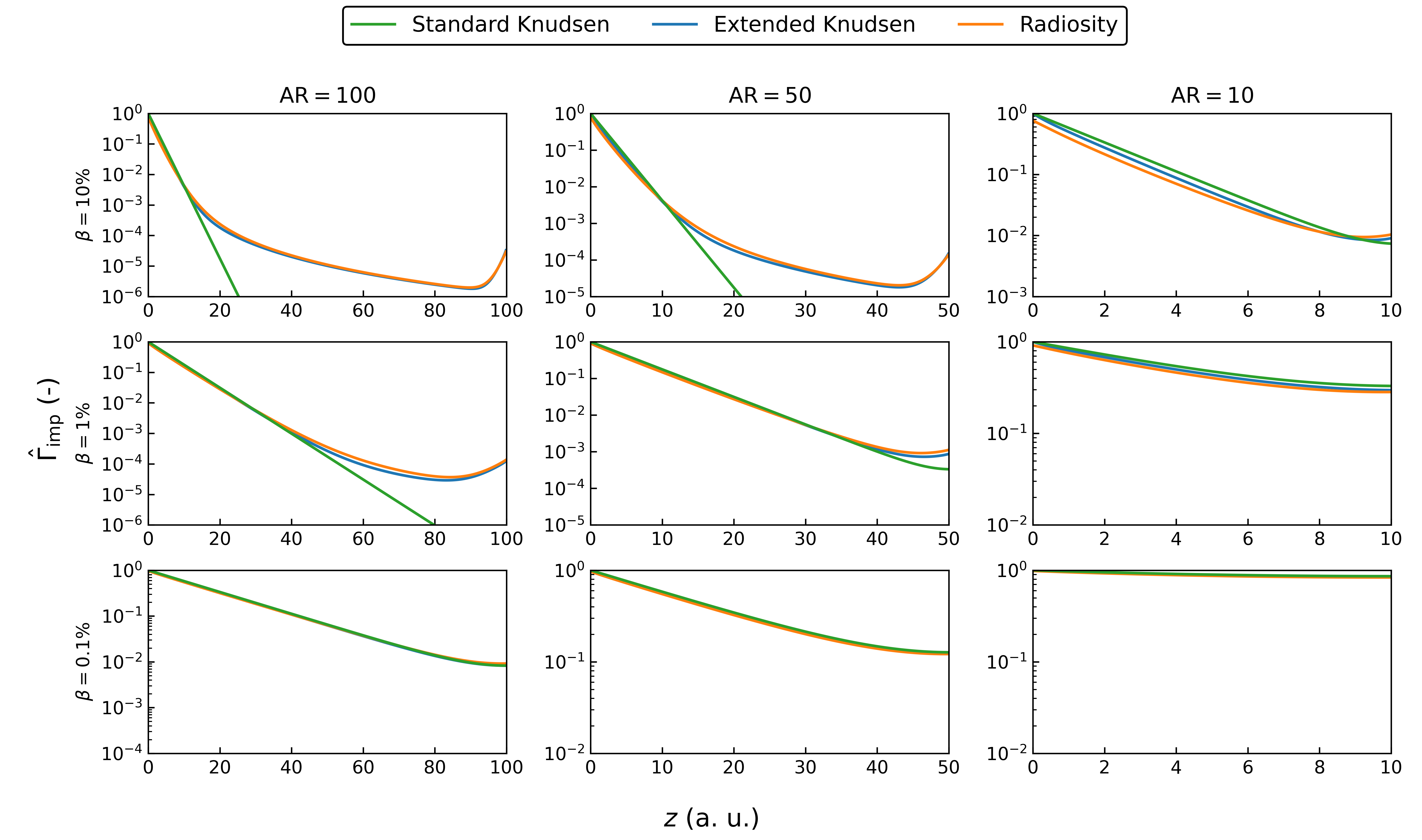
Figure 3.8: Comparison of normalized impinging flux \(\hat {\Gamma }_\mathrm {imp}\) calculated using extended Knudsen diffusion to that using standard Knudsen and the radiosity framework [108] as a function of the
axial distance \(z\) in arbitrary units. Calculations were performed for a finite cylinder of diameter \(d=\SI {1}{\arbitraryunit }\) for multiple values of constant sticking coefficient \(\beta \) and aspect ratio AR.
In Fig. 3.8, it can be seen that the extended Knudsen diffusion follows very closely the curve obtained using the radiosity framework. Since the latter evaluates the
integral equation and has been validated with a Monte Carlo simulation [108], it can be considered the exact result for a cylinder. For cylinders with low \(\beta \), all flux calculations yield very similar results which is
expected from the characteristics of Knudsen diffusion discussed so far. Interestingly, qualitatively similar results among all calculations are also obtained for the lowest AR cylinder, even though the standard Knudsen diffusion has
been constructed for long cylinders. This is evidence that, for relatively short cylinders, the important physical phenomena are captured by the boundary conditions instead of the diffusivity.
In the situation of high AR and high \(\beta \), standard Knudsen diffusion deviates more notably from both extended Knudsen diffusion and the radiosity framework. This is due to the lack of direct flux in standard Knudsen
diffusion, thus the exponential decline of Eq. (3.31) is the only dominating factor. Naturally, in situations of higher \(\beta \),
attention must be placed on the role of the direct flux. A methodology to partially recover the effects of the direct flux while still using the standard Knudsen diffusion is discussed in Section 3.6.2.
Nonetheless, the success of the extended Knudsen diffusion should be carefully interpreted. The qualitative agreement shown in Fig. 3.8 is an indication of the small
relative error between the extended diffusive calculations and the exact radiosity framework. However, since \(\hat {\Gamma }_\mathrm {imp}\) is already normalized to \(\Gamma _\mathrm {source}\), it is in fact more useful
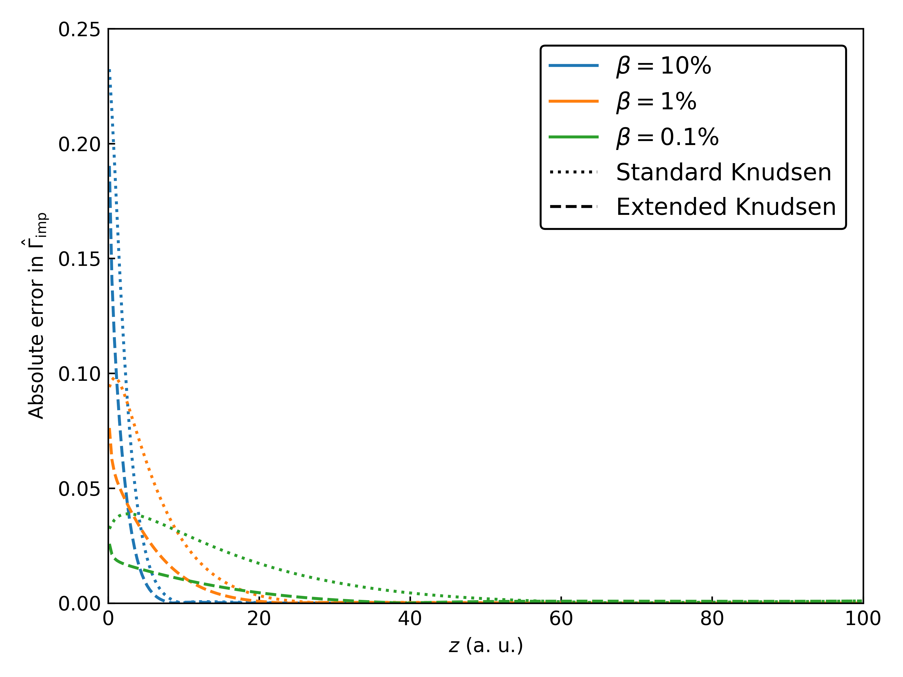
to focus on the absolute error in \(\hat {\Gamma }_\mathrm {imp}\) to obtain the deviation in units of \(\Gamma _\mathrm {source}\). This is shown in Fig. 3.9 for the case of a cylinder of \(d=\SI {1}{\arbitraryunit }\) and \(\text {AR}=100\). There, it can be seen that the error is more pronounced at the top of
the cylinder for higher values of \(\beta \). Such error is likely a consequence of the boundary condition in Eqs. (3.29) and (3.50) imposing maximum flux at the top. For higher values of \(\beta \), the reduction in flux due to the \(\SI {90}{\degree }\) inclination of the cylinder wall with
respect to the source plane is an important factor which is not captured.
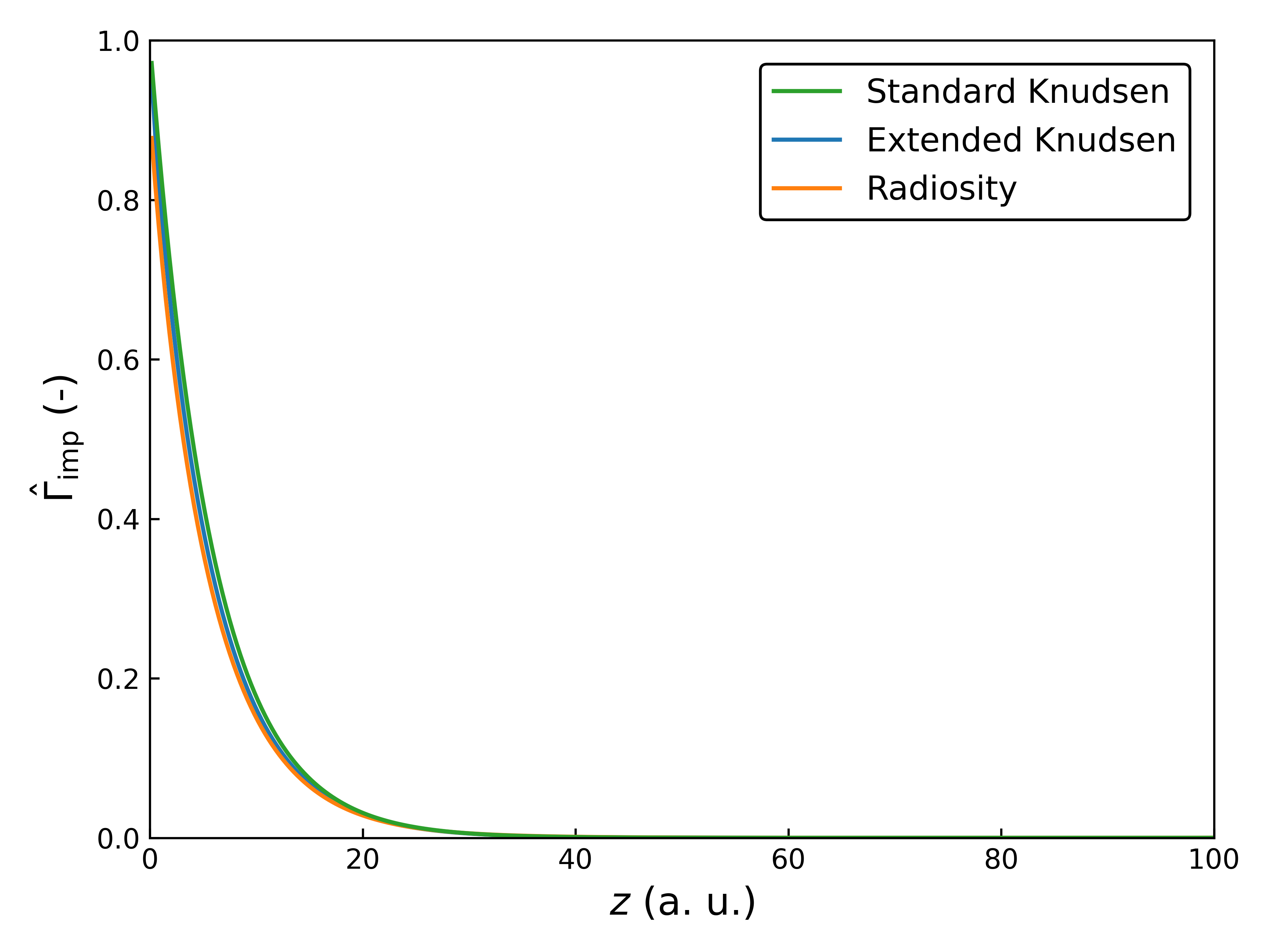
Additionally, the difference in absolute error between the standard and extended Knudsen diffusion is minimal. This is more apparent when one of the results from Fig. 3.8 is evaluated without the logarithmic scale. This is shown in Fig. 3.10 for the cylinder with
\(\text {AR}=100\) and \(\beta =1\,\%\). In this linear plot, it is clear that all curves are very similar qualitatively. Therefore, the standard Knudsen approach is more than adequate for many applications, as long as the
phenomenological parameters are sufficiently adjusted.
Figure 3.9: Axial length (\(z\)) distribution of the absolute error of extended and standard Knudsen diffusion compared to the exact radiosity framework [108] for a finite cylinder with \(d=\SI {1}{\arbitraryunit }\) and
\(\text {AR}=100\) for multiple values of \(\beta \).
Figure 3.10: Linear scale comparison of extended Knudsen diffusion to standard Knudsen and the radiosity framework [108]. Calculations were performed for a finite cylinder with \(d=\SI {1}{\arbitraryunit }\), \(\text
{AR}=100\), and \(\beta =1\,\%\).