As introduced in Section 4.1, there exists a wealth of complex chemistry in ALP. In order to develop a model which might be applied to real high AR structures, this complexity
must be encapsulated in a simpler phenomenological model, since the underlying quantum chemical reality cannot be modeled at such large scale [153, 154]. To illustrate the construction of phenomenological first-order
Langmuir surface kinetics, the H2O step of the ALD of Al2O3 is taken as an example. Figure 4.2 depicts the three reaction
pathways considered by such a model: An incoming H2O molecule can either adsorb or reflect upon interacting with the surface, mediated by the coverage-dependent sticking coefficient \(\beta (\Theta )\) from
Eq. (2.4). In addition, an already adsorbed molecule is allowed to spontaneously desorb given a fixed evaporation flux \(\Gamma _\mathrm {ev}\).
Under the additional assumption that the H2O supply is the only limiting factor (i.e., \(\Theta _\mathrm {TMA}(\vec {r}){=}1\)), the state of the surface is fully determined by the distribution of the
H2O coverage \(\Theta _\mathrm {H_2O}(\vec {r})\) given by Eq. (2.3). That is, the particle involved in the reactive
transport is the limiting chemical reactant. The complex chemical behavior is then condensed into two phenomenological parameters: \(\beta _0\) and \(\Gamma _\mathrm {ev}\). The challenge with solving Eq. (2.3) is that it depends on the impinging water flux \(\Gamma _\mathrm {imp}\) which itself depends on the surface state according to \(\beta
(\Theta )\).
To break this loop, Eq. (2.3) is discretized using the forward Euler method up to the pulse time \(t_p\), obtaining
\(\seteqnumber{0}{4.}{4}\)
\begin{align}
\label {eq::discretized_langmuir} \Theta ^{n+1}_\mathrm {H_2O}(\vec {r}) = \Theta ^n_\mathrm {H_2O}(\vec {r}) + h_t s_0 \Gamma _\mathrm {imp,H_2O}^n(\beta (\Theta ^n_\mathrm {H_2O}),\vec {r})
\beta _0 (1-\Theta ^n_\mathrm {H_2O}(\vec {r})) - h_t s_0 \Gamma _\mathrm {ev} \Theta ^n_\mathrm {H_2O}(\vec {r})\, ,
\end{align}
where \(n\) is a time integration index going from \(0\) to \(N_t\) total steps, such that the time step length is \(h_t = t_p/(N_t+1)\). The initial condition is \(\Theta ^0_\mathrm {H_2O}(\vec {r}){}=0\). Assuming that
the \(\Gamma _\mathrm {imp,H_2O}\) is normalized to \(\Gamma _\mathrm {source}\) according to Eq. (2.7), a simple estimation for the
stability of Eq. (4.5) is:
\(\seteqnumber{0}{4.}{5}\)
\begin{align}
\label {eq::langmuir_stability} h_t < \frac {1}{s_0 \left (\beta _0 \Gamma _\mathrm {source} + \Gamma _\mathrm {ev} \right )}
\end{align}
The surface site area \(s_0\) can be calculated from the stoichiometric ratio between the number of deposited atoms present in the reactant formula to those in the film formula \(b_\mathrm {reactant}/b_\mathrm {film}\), the
film mass density \(\rho \), the film molar mass \(M\), the GPC, and Avogadro’s constant \(N_0\) as [109]
\(\seteqnumber{0}{4.}{6}\)
\begin{align}
\label {eq::s_0} s_0 = \frac {b_A}{b_\mathrm {film}}\frac {M}{N_0 \cdot \text {GPC}\cdot \rho }\, .
\end{align}
For the H2O step of the ALD of Al2O3, \(b_\mathrm {H_2O}/b_\mathrm {Al_2O_3} = 1/3\), and the remaining factors can be experimentally measured and are usually reported. It is
important to note that Eq. (4.7) is only an approximation to the surface site area, since, e.g., the effects of steric hindrance [68] are not included.
Although the discretization from Eq. (4.5) solves the issue of the coupling between reactant transport and surface chemistry, it does so at the
cost of performing the transport calculation \(N_t\) times per advection step. In topography simulations of conventional processes such as reactive ion etching (RIE), the involved Langmuir equations are assumed to be on the
steady-state [41, 43], thus only a single transport calculation is required per advection step. Therefore, the use of an accurate top-down pseudo-particle tracking approach to \(\Gamma _\mathrm {imp}\), presented in
Section 2.3.3, can be exceedingly demanding for computational resources. Nonetheless, the use of Monte Carlo pseudo-particle tracking has been reported for ALD [101, 155].
To avoid this large computational cost and, therefore, to enable more efficient investigations of the effect of the parameters an one-dimensional (1D) diffusive model can be used. The approach of combining Knudsen diffusion and
Langmuir kinetics has been first introduced for ALD by Yanguas-Gil and Elam [30, 111, 124]. However, their approach assumes irreversible adsorption, i.e., \(\Gamma _\mathrm {ev}{=}0\). According to the formulation of
Chapter 3, the diffusive reactive transport ordinary differential equation (ODE) in the preferential transport direction \(z \in [0,L]\) can be written as follows:
The formulation in Eq. (4.8), differently than that from [124], enables more versatility in the calculation of \(D\). The diffusivity can be calculated
not only via the standard Knudsen diffusivity from Eq. (3.24), but it can also include the geometric factors for
rectangular trenches discussed in Section 3.3, as well as transitional flow through the Bosanquet interpolation formula from Eq. (3.44). The thermal speed \(\overline {v}\) is calculated using the reactor temperature and reactant molar mass using Eq. (3.4). The source flux \(\Gamma _\mathrm {source}\) is inferred from the reactant partial pressure using the Hertz-Knudsen relationship from Eq. (3.7).
Equations (4.8) to (4.10) require a numerical solution.
They are solved using a central finite differences scheme by dividing the \(z\) domain in \(N_z+1\) slices of size \(h_z=L/(N_z+1)\) and index \(k\). The following tridiagonal equation system is obtained:
The crucial assumption behind phenomenological modeling is that the model parameters, namely \(\beta _0\) and \(\Gamma _\mathrm {ev}\), are strongly correlated to the reactor conditions. Therefore, before moving to the
parameter investigations with support of experimental data in Section 4.4, it is important to investigate the effects of the model parameters over conformality. To quantify conformality,
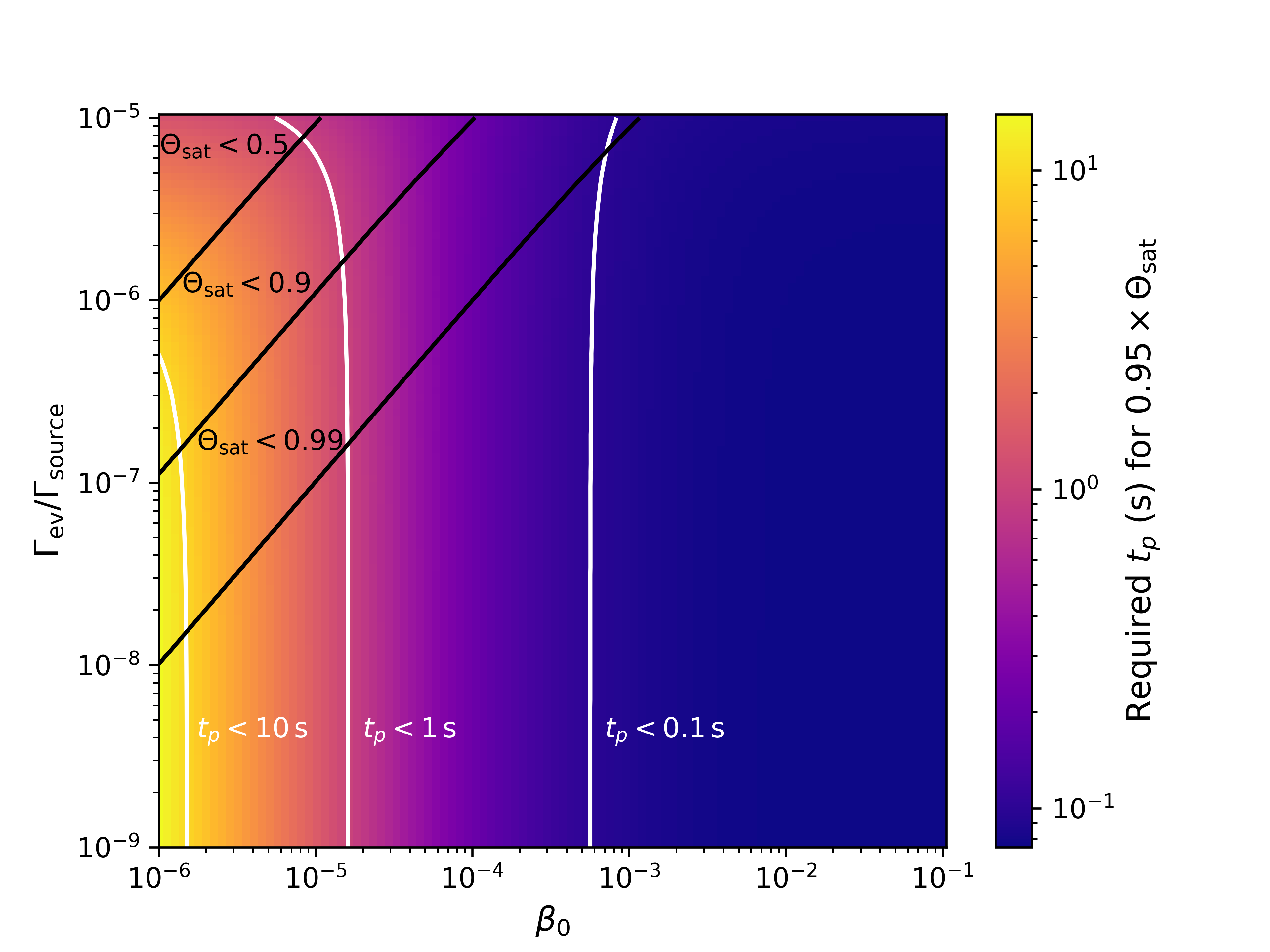
two calculations are performed for each pair of parameters. First, the saturation coverage \(\Theta _\mathrm {sat}\) is calculated at \(z{=}L\) as the steady-state convergence (\(d\Theta /dt=0\)) of Eq. (4.5). Then, a second calculation is performed, now to calculate the required \(t_p\) to achieve \(95\%\) of \(\Theta _\mathrm {sat}\). A region
of the parameter space is shown in Fig. 4.3, calculated with standard Knudsen diffusivity for a cylinder with \(d = \SI {1}{\micro \meter }\) and \(L = \SI
{100}{\micro \meter }\), and a fictitious reactor chemistry with \(s_0 = \SI {2e-19}{\meter ^{-2}}\) and \(\Gamma _\mathrm {source} = \SI {e24}{\meter ^{-2}\second ^{-1}}\).
Figure 4.3 indicates that the required \(t_p\) is mostly impacted by the \(\beta _0\) parameter, as the gradient varies little across the \(y\) axis. Instead, the impact of
\(\Gamma _\mathrm {ev}\) is on restricting the maximum achievable \(\Theta _\mathrm {sat}\), as seen in the upper left-hand side of the figure. That is, \(\Gamma _\mathrm {ev}\) severely limits the maximum AR which can
be conformally processed by an ALP reactor configuration, even for values as low as one millionth of \(\Gamma _\mathrm {source}\).