Phenomenological Single-Particle
Modeling of Reactive Transport
in Semiconductor Processing
3.6 Applications
In this section, two hitherto unpublished applications of Knudsen diffusive transport are presented. Both of them are direct applications of the standard Knudsen diffusion derived in Section 3.2 under the approximation of constant \(\beta \). Section 3.6.1 presents an analysis of AR dependent phenomena in RIE through a direct integration of \(\hat {\Gamma }_\mathrm {imp}\), while Section 3.6.2 presents a variation of standard Knudsen diffusivity including the direct flux more directly than the presentation in Section 3.5. The latter is applied to model heteroepitaxial growth of cubic silicon carbide (3C-SiC) on silicon (Si).
3.6.1 Aspect Ratio Dependent Reactive Ion Etching
RIE is a plasma processing technique which enables etching of high AR structures [129]. This is achieved through the combination of at least two different reactants: Neutrals and ions. It is known since the groundbreaking work by Coburn and Winters [130] that the combined etch rate due to both neutrals, such as chlorine gas (Cl2), and ions, like argon (Ar+ ), is much higher than their individual contributions. Since the ions are vertically accelerated due to the plasma sheath, this enables a considerable vertical etch and, thus, the etching of high AR structures.
However, since there is a nonzero lateral component due to the neutrals which are not vertically accelerated, additional chemical reactions were developed to passivate the sidewalls [131]. For example, fluorocarbon containing plasmas naturally deposit a C\(_x\)F\(_y\) polymer layer which protects the surface from etching. The reactor is then fine-tuned so that the neutrals are unable to strip the polymer layer by themselves. Instead, only the bottom has the protective polymers removed, since it is affected by both neutrals and ions. This increased selectivity due to sidewall passivation enables even higher ARs. Therefore, ever more complex modeling flux models, with a precise description of the three involved reactant species, are required to accurately reproduce experimental topographies [43, 132].
The further development of RIE requires tremendous engineering effort to overcome its grand challenges [133]. From those many challenges, one crucial issue which must be addressed is that of aspect ratio dependent etching (ARDE): An observed reduction in etch rates as the AR increases. This phenomenon can have multiple overlapping causes [134], such as ion shading, bulk or surface diffusion, or even electric charge effects. However, the cause which has received the most research attention has been the restricted transport of neutral species towards the bottom of the feature [129].
This situation of restricted neutral transport is an ideal candidate for investigation of the so far discussed Knudsen diffusivity, so much so that it is usually named "Knudsen transport" in the literature [134]. In order to reduce the complex RIE problem to a single representative particle, a few assumptions about the process must be made. Firstly, it is assumed that the ion transport is perfectly vertical. That is, it does not affect vertical sidewalls and the ion flux at the bottom is independent of the AR. This vertical ion transport also completely removes any possible passivation layers at the bottom.
Thus, both the sidewall and the bottom may have different chemical compositions which are approximately represented by the respective constant sticking coefficients \(\beta _\mathrm {wall}\) and \(\beta _\mathrm {bottom}\). This assumption means that the sidewalls are uniformly coated with an infinitesimally thin protective film and the bulk material at the bottom is fully exposed. Since there are now two involved sticking coefficients, the ODE and necessary BCs for \(\hat {\Gamma }_\mathrm {imp}(z)\) in a cylinder with diameter \(d\), first presented in Section 3.2, now take the form:
\(\seteqnumber{0}{3.}{53}\)\begin{align} \label {eq::ARDRIE_ODE} \frac {d^2 \hat {\Gamma }_\mathrm {imp}}{dz^2} =&\, \frac {3}{d}\beta _\mathrm {wall} \hat {\Gamma }_\mathrm {imp}(z) \\[1em] \label {eq::ARDRIE_first_BC} \hat {\Gamma }_\mathrm {imp}(0) =&\, 1 \\[1em] \label {eq::ARDRIE_second_BC} \left . \frac {d \hat {\Gamma }_\mathrm {imp}}{dz} \right |_{z=L} =&\, \frac {3}{4d}\beta _\mathrm {bottom}\hat {\Gamma }_\mathrm {imp}(L) \end{align}
Equation (3.54) has the exact solution:
\(\seteqnumber{0}{3.}{56}\)\begin{align} \label {eq::ARDRIE_solution} \hat {\Gamma }_\mathrm {imp} = e^{-\frac {z \sqrt {3\beta _{\mathrm {wall}}}}{d}} \frac { 3 \beta _{\mathrm {bottom}} \left (e^{\frac {2 L \sqrt {3 \beta _{\mathrm {wall}}}}{d}}{-} e^{\frac {2 z \sqrt {3 \beta _{\mathrm {wall}}}}{d}}\right )+4 \sqrt {3 \beta _{\mathrm {wall}}} \left ( e^{\frac {2 L \sqrt {3\beta _{\mathrm {wall}}}}{d}}{+}e^{\frac {2 z \sqrt {3\beta _{\mathrm {wall}}}}{d}}\right )}{3 \beta _{\mathrm {bottom}}\left (e^{\frac {2 L \sqrt {3\beta _{\mathrm {wall}}}}{d}}{-}1\right ) +4 \sqrt {3\beta _{\mathrm {wall}}} \left ( e^{\frac {2 L \sqrt {3\beta _{\mathrm {wall}}}}{d}}{+}1\right )} \end{align} Since Eq. (3.57) is numerically unstable in the limit \(\beta _\mathrm {wall}\to 0\), due to it approaching \(0/0\), an exact solution can be directly obtained from Eq. (3.54) for \(\beta _\mathrm {wall}=0\):
\(\seteqnumber{0}{3.}{57}\)\begin{align} \label {eq::ARDRIE_solution_zero} \hat {\Gamma }_{\mathrm {imp},\beta _\mathrm {wall}=0} = \frac {4d + 3 \beta _\mathrm {bottom} (L-z)}{4d + 3 \beta _\mathrm {bottom} L} \end{align}
The empirical observation of ARDE is that, as the AR increases, the etch rate decreases. However, in many cases what is measured is not the instantaneous etch rate. Instead, the etch time \(t_\mathrm {etch}\) and plane wafer etch rate PWR are usually well-defined, leading to an expected ideal etch depth \(L_\mathrm {ideal}=t_\mathrm {etch}\cdot \mathit {PWR}\). The observation is then of a reduced etch depth \(L_\mathrm {ARDE}\) due to ARDE which can in turn be empirically related to etch rates. Nonetheless, the derived Eqs. (3.57) and (3.58) enable the direct calculation of \(L_\mathrm {ARDE}\) which, additionally to providing insight into the ARDE phenomenon, also enables the single-step simulation of topographies through Boolean operations [48].
Since the RIE is assumed to be limited by a single species, \(L_\mathrm {ARDE}\) can be calculated from the impinging flux at the bottom of the feature \(L\) at each time step and the definition of PWR from Eq. (2.8):
\(\seteqnumber{0}{3.}{58}\)\begin{align} \label {eq::L_ARDE} L_\mathrm {ARDE} = \int _0^{t_\mathrm {etch}} v(z{=}L,t)dt = \int _0^{t_\mathrm {etch}} \hat {\Gamma }_\mathrm {imp}(L)\cdot \mathit {PWR}\,dt = \int _0^{L_\mathrm {ideal}} \hat {\Gamma }_\mathrm {imp}(L)dL \end{align} Equation (3.59) has the following solution for the nonzero \(\beta _\mathrm {wall}\) case
\(\seteqnumber{0}{3.}{59}\)\begin{align} \label {eq::L_ARDE_constant} L_\mathrm {ARDE} = \frac {8d}{4\beta _\mathrm {bottom}+ 4\sqrt {3\beta _\mathrm {wall}}}A\left [ \arctan {\left (Ae^{\frac {L_\mathrm {ideal}\sqrt (3\beta _\mathrm {wall})}{d}}\right )-\arctan {A}} \right ]\, , \end{align} where
\(\seteqnumber{0}{3.}{60}\)\begin{align} \label {eq::L_ARDE_A} A = \sqrt {\frac {16 \beta _{\text {wall}}-3 \beta _{\mathrm {bottom}}^2}{16 \beta _{\text {wall}} + 3 \beta _{\mathrm {bottom}}^2-8 \beta _{\mathrm {bottom}} \sqrt {3\beta _{\text {wall}}}}}\, . \end{align} For the zero \(\beta _\mathrm {wall}\) case, the expression takes the simpler form
\(\seteqnumber{0}{3.}{61}\)\begin{align} \label {eq::L_ARDE_zero} L_{\mathrm {ARDE},\beta _\mathrm {wall}=0} = \frac {4d}{3\beta _\mathrm {bottom}}\ln {\left (1+\frac {3L_\mathrm {ideal}\beta _\mathrm {bottom}}{4d}\right )}\, . \end{align}
With these expressions having been derived, it is now possible to precisely evaluate the impact of the restricted neutral impact with the increase of AR. To that end, a measure of etch depth attenuation due to ARDE is defined as \({L_\mathrm {ARDE}}/{L_\mathrm {ideal}}\). Both the attenuation and the achieved AR can be calculated for varying values of \(L_\mathrm {ideal}\), representing the effect of increasing the \(t_\mathrm {etch}\). These results are shown in Fig. 3.11 for a cylinder of diameter \(d=\SI {1}{\arbitraryunit }\) and \(\beta _\mathrm {bottom}=1\,\%\).
In Fig. 3.11, it can be seen that the attenuation is very sensitive to \(\beta _\mathrm {wall}\). In fact, for all positive values of \(\beta _\mathrm {wall}\), it can be seen that the AR reaches a finite value. This is an indication that the interactions between the neutral etchants and the polymer film, here described \(\beta _\mathrm {wall}\), must be very carefully engineered to enable higher ARs. If this is not carefully considered, the standard approaches of increasing reactor pressure and \(t_\mathrm {etch}\) to overcome ARDE [129] will be fruitless.

Notably, by calculating the limit \(L_\mathrm {ideal} \to \infty \) for \(L_\mathrm {ARDE}\) in Eq. (3.60) and dividing it by \(d\), an expression for the maximum achievable AR which does not depend on \(d\) can be obtained. This limit is plotted in Fig. 3.12, where the interplay between \(\beta _\mathrm {wall}\) and \(\beta _\mathrm {bottom}\) can be evaluated. Although a \(\beta _\mathrm {wall}\) far below \(0.01\,\%\) is strictly necessary for enabling features with AR above \(100\), engineering effort must also be put at the interaction between the reactant and the exposed bottom surface. Nonetheless, the limit calculation of the maximum achievable AR diverges for \(\beta _\mathrm {wall}=0\) but not for \(\beta _\mathrm {bottom}=0\), therefore, the ultimate enabler of very high AR is the control over the interactions with the sidewall material.

3.6.2 Heteroepitaxial Growth of 3C-SiC on Si
3C-SiC is a promising material for power electronic applications, in particular in the \(600{-}\SI {1200}{\volt }\) range [135]. Although the 4H-SiC allotrope has found more widespread commercial application [136], it is usually applied to a higher voltage range. To enable the further development and implementation of 3C-SiCs technology, the open scientific question of growing high-quality 3C-SiC substrates must be addressed. This material cannot be heteroepitaxially grown on a standard plane Si wafer without large defects due to the large lattice mismatch, even for comparatively more compatible Si(\(111\)) wafers [137].
To bridge this gap and enable highly crystalline 3C-SiC within the framework of well-established Si wafer technology, a methodology involving micro-pillars has been proposed by Kreiliger et al. [138]. In their methodology, hexagonal arrays of micro-pillars are etched on a Si(\(111\)) wafer using deep reactive ion etching (DRIE). Then, 3C-SiC is heteroepitaxially grown on top of these micro-pillars using a low-pressure CVD reactor with ethylene (C2H4) and trichlorosilane (TCS) as reactants. By carefully engineering the dimensions and spacing of the micro-pillars, defects can be minimized, since the growing crystals coalesce into a continuous layer in a manner which is more favored by the lattice structure.
As there is a large degree of required optimization of the involved geometry, in particular with respect to the interaction between the shape of the micro-pillar and the crystal-direction dependent growth of 3C-SiC, topography simulation can play a helpful role. Previously, a detailed phase-field approach to model growth and coalescence has been proposed [139]. This model involves effects which are commonly not integrated within level-set (LS) based topography simulation, notably surface diffusion. However, the impinging reactant fluxes are modeled by assuming a combination of vertical and isotropic components. This is unusual for CVD processes since, as discussed in Chapter 2, the reactants are assumed to be isotropically distributed if no acceleration mechanism, such as a plasma sheath, is present [30].
This motivates the development of a simple reactive transport model in order to model this growth process with the LS method. Similarly to the case of anisotropic wet etching described in Section 2.3.1 and to LS modeling of solid phase epitaxial regrowth (SPER) [140], a crystallographic-orientation dependent (i.e., surface normal \(\vec {n}\) dependent) velocity field \(v_\mathrm {crystal}(\vec {n})\) can be built via interpolation of calibrated growth rates \(R_m\) for each involved crystal plane \(m\) [87, 141]. However, since a low-pressure CVD reactor is inherently transport-controlled, the growth rate must be modulated by a local impinging flux
\(\seteqnumber{0}{3.}{62}\)\begin{align} \label {eq::growth_flux_epitaxy} v(\vec {r},t) = \hat {\Gamma }_\mathrm {imp}(\vec {r}) \cdot v_\mathrm {crystal}(\vec {n}(\vec {r}))\, , \end{align} where \(v_\mathrm {crystal}(\vec {n}(\vec {r}))\) is given by Eq. (2.9). The development and calibration of \(v_\mathrm {crystal}(\vec {n})\) was performed by the colleague Alexander Toifl of the Christian Doppler Laboratory for High Performance Technology Computer-Aided Design (HPTCAD), while the development of the local impinging flux model is the focus of this thesis.
From a visual analysis of the reported growth profiles in [139], it can be noted that the majority of the growth occurs at the top of the pillar, however, with some infiltration present below the maximum lateral extent. This indicates that the involved reactants have a high but not \(100\,\%\) sticking coefficient \(\beta \), since there is growth in regions not directly visible to the reactor. Therefore, the direct flux must be taken into account in combination with the infiltration process which can be interpreted as Knudsen diffusion. To efficiently model this combination of factors without recurring to the complex calculations from, e.g., Section 3.5, the impinging flux can be divided into a sum of two components. One is due to the direct flux \(\hat {\Gamma }_\mathrm {direct}\) which can be calculated using the bottom-up approach discussed in Section 2.3.2 and the efficient algorithms present in Silvaco’s Victory Process [55], and the other is the Knudsen flux \(\hat {\Gamma }_\mathrm {Kn}\). These components are combined via
\(\seteqnumber{0}{3.}{63}\)\begin{align} \label {eq::combined_direct_knudsen} \hat {\Gamma }_\mathrm {imp} = B\cdot \hat {\Gamma }_\mathrm {direct} + (1-B)\cdot \hat {\Gamma }_\mathrm {Kn}\, , \end{align} where \(B\) is a model parameter which dictates the relative strength of the direct flux component. \(B\) can be interpreted as a rough approximation to \(\beta \), assuming a single effective particle.
The evaluation of \(\hat {\Gamma }_\mathrm {Kn}\) for evolving micro-pillars poses a specific set of problems. The central issue is that it is not straightforward to map from the dynamically evolving micro-pillar to an equivalent cylinder, which is the reference for the Knudsen diffusion equations derived so far. Although an EAR has been proposed for square pillars [110], its value is not rigorously calculated. Instead, the calculation of \(\hat {\Gamma }_\mathrm {Kn}\) for the involved micro-pillars is done by directly considering the Thiele modulus \(h_T^2\) from Eq. (3.27) as a model parameter. Since \(h_T^2\) represents the ratio of the reaction rate to the transport rate [50, 124], this is a considerably coarse approximation. In essence, it is assumed that the transport rate is constant as the pillars coalesce, that is, the increased constriction due to coalescence is disregarded. Also, both reactants are jointly approximated by a single effective particle with a fixed reaction rate. This leads to the modeling ODE:
\(\seteqnumber{0}{3.}{64}\)\begin{align} \label {eq::3C-SiC_ODE} \frac {d^2 \hat {\Gamma }_\mathrm {Kn}}{d z^2} = h_T^2 \hat {\Gamma }_\mathrm {Kn}(z) \end{align} To evaluate Eq. (3.65), two BCs are necessary. Instead of setting the reactor supply boundary condition at a fixed plane \(z{=}0\), a boundary plane \(z_0\) is dynamically extracted from the simulated topography. The \(z_0\) plane is defined as that for which the maximum lateral (\(x\),\(y\)) extent is achieved. That is, only below the \(z_0\) plane the Knudsen diffusion processes takes place, as it is the region where multiple particle-geometry interactions are more likely to happen due to constriction. The reactor efficiency boundary condition then becomes
\(\seteqnumber{0}{3.}{65}\)\begin{align} \label {eq::3C-SiC_first_BC} \hat {\Gamma }_\mathrm {Kn}(z{\ge }z_0) = 1\, . \end{align} Additionally, unlike Section 3.6.1, the flux near the bottom of the micro-pillar is of little importance, since no growth is experimentally observed there. Thus, to obtain a simpler expression which captures the essentials of the exponential behavior from Fig. 3.10, a simpler "bottomless" BC is employed
\(\seteqnumber{0}{3.}{66}\)\begin{align} \label {eq::3C-SiC_second_BC} \lim _{z \to -\infty }{\hat {\Gamma }_\mathrm {Kn}(z)}=0 \end{align} Therefore, the Knudsen flux has a straightforward exact solution:
\(\seteqnumber{0}{3.}{67}\)\begin{align} \label {eq::3C-SiC_flux} \hat {\Gamma }_\mathrm {Kn} = \begin{cases} 1, & z \ge z_0 \\ e^{h_T(z-z_0)}, & z < z_0 \end {cases} \end{align}
This model has been implemented within Victory Process [55] and calibrated to the reported profiles from Masullo et al. [139]. The calibrated parameters are reported in Tab. 3.1. The results of the simulated topography after \(\SI {60}{\minute }\), including the time evolution of the facets and the comparison to the experimentally measured profiles, are shown in Fig. 3.13.
| Thiele modulus | Direct flux component | Crystal growth rates [\(\si {\micro \meter /\hour }\)] | ||||
| \(h_T\) | \(B\) |
|
||||
| 0.5 | 0.7 |
|
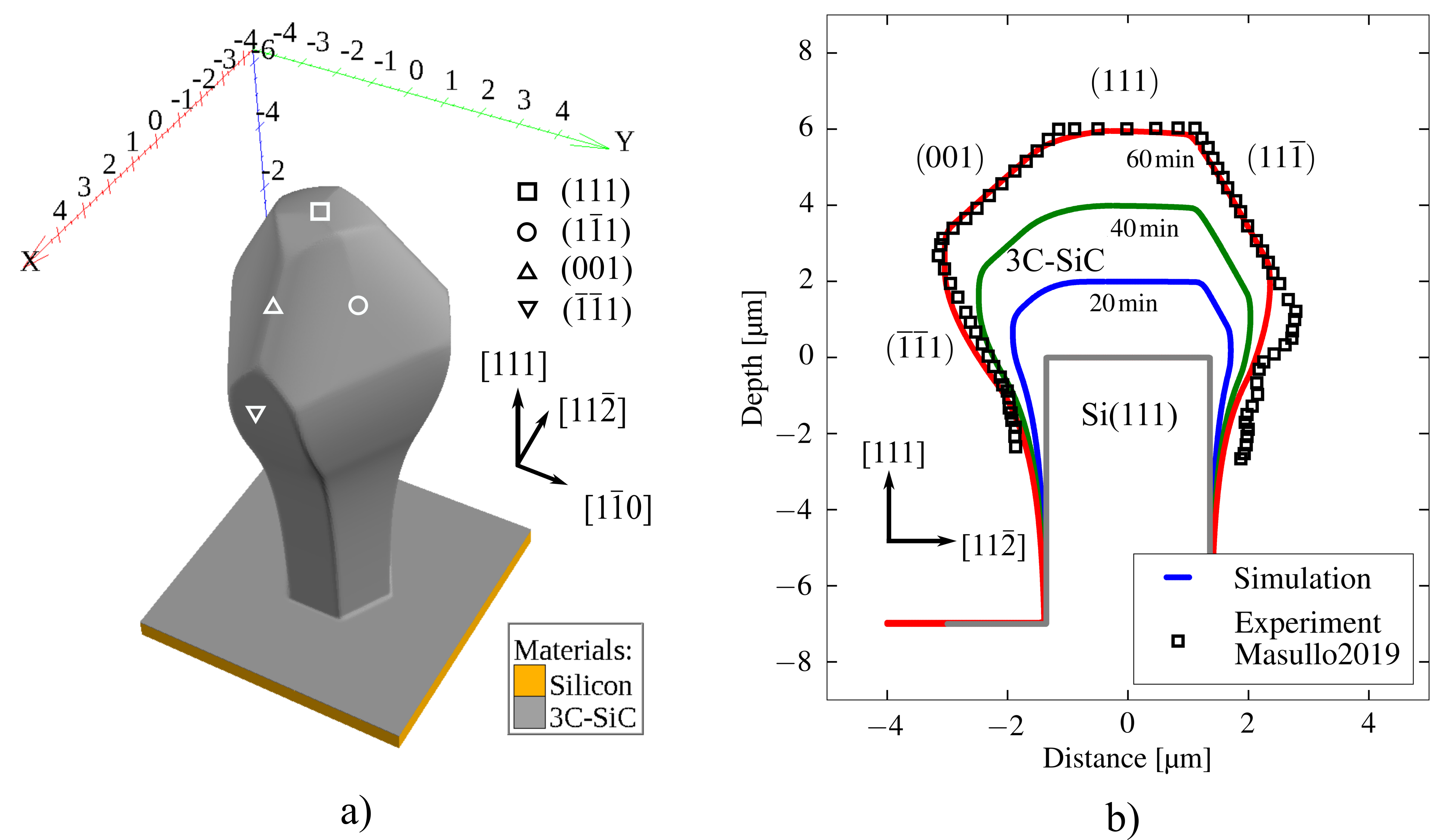
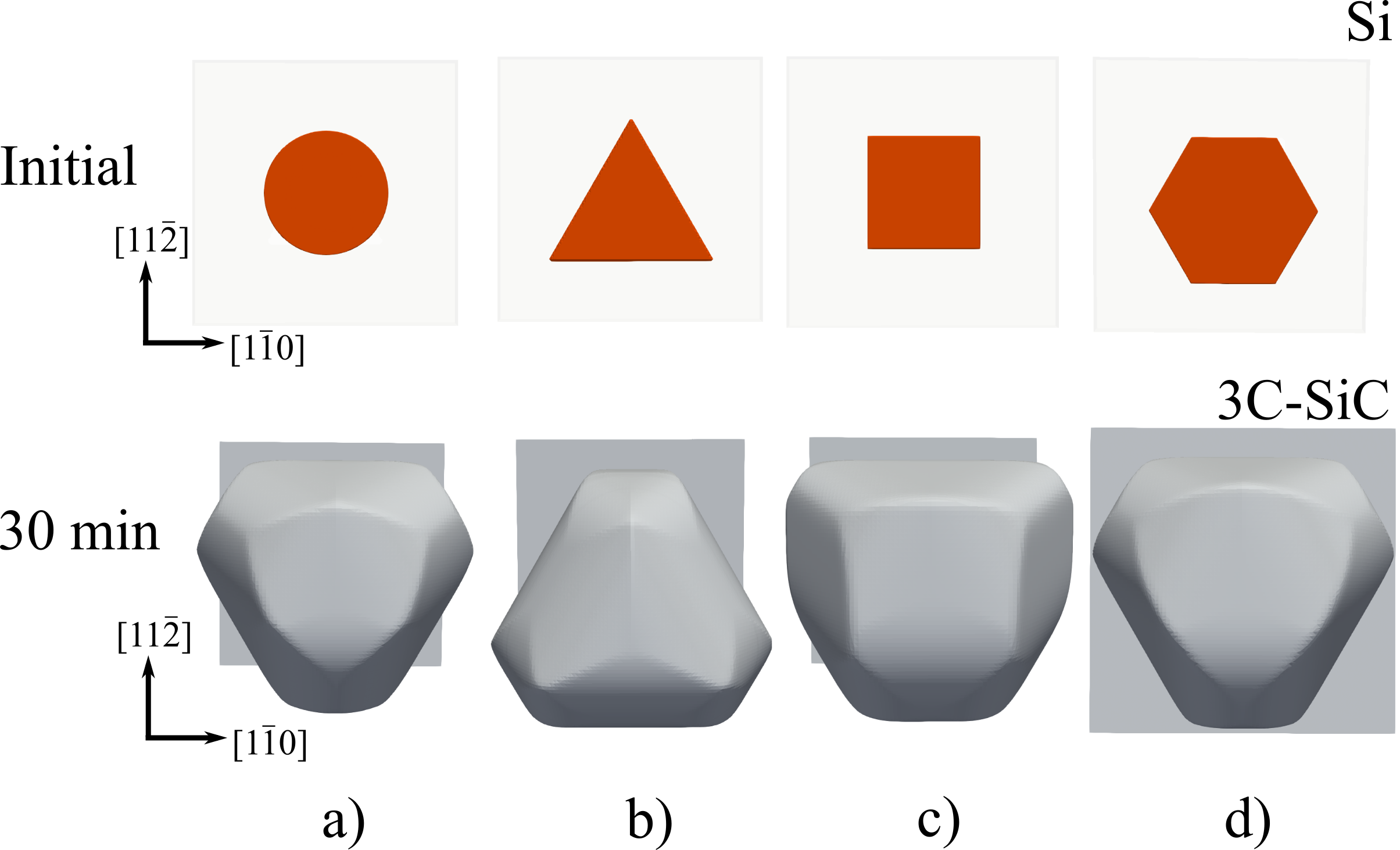
Figure 3.13 shows good agreement between the model combining both direct and Knudsen flux with the reported experiment, even after the use of rather coarse approximations. This is evidence that either the surface diffusion is not a critical determinant of the final profile, or that this process is effectively captured by the crystallographic growth rates \(R_m\) and the interpolation procedure. The discrepancy seen on the right-hand side of Fig. 3.13.b) is likely due to the use of a single boundary plane \(z_0\) at an excessively high position, as \(z_0\) is determined by the shape on the left-hand side of the image. Therefore, the flux is artificially restricted on the right-hand side. This can be alleviated by extracting a separate value of \(z_0\) for each (\(x\),\(y\)), or by a more accurate calculation approach such as the top-down tracking discussed in Section 2.3.3. Nonetheless, the success of the simulation means that it can be used for exploring different micro-pillar geometries. This is shown in Fig. 3.14 for simulated crystals after \(\SI {30}{\minute }\) growth on four initial geometries, highlighting a path for future optimization.