Phenomenological Single-Particle
Modeling of Reactive Transport
in Semiconductor Processing

6.3 Optical Parameter Extraction

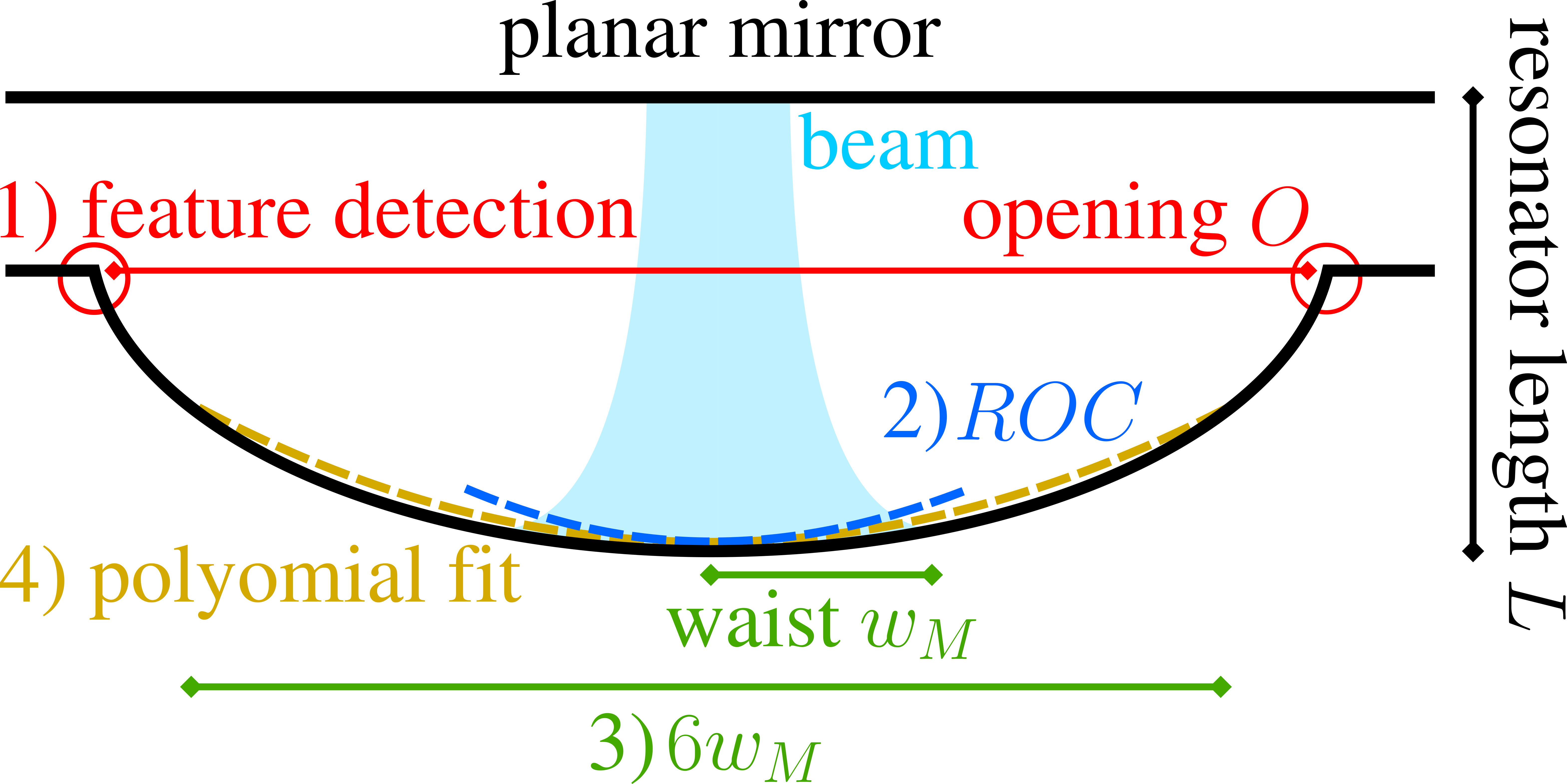
The feature detection procedure described in Section 6.2 is sufficient for determining a thorough description of a single cavity. However, to understand the impact of the quality of the microcavity on the assembled resonator, the entire device must be considered. Through Gaussian beam analysis of an assembled resonator [187], optical parameters can be extracted in a rough approximation of a device simulation, as they are representative of possible device performance. For simplicity, a PC resonator is considered, which is shown in Fig. 6.6 together with the extraction procedure of such parameters.

The starting point of the optical parameter extraction procedure is the feature detection algorithm, first presented in Section 6.2. Having obtained the maximum cavity opening \(O\) and having projected the data onto the radial coordinate, a representative ROC is extracted by fitting a parabola \(y = ax^2+c\) to the central \(50\,\%\) of the maximum opening. This restriction is necessary to have an accurate parabolic fit, since the shape might deviate from an ideal parabola if the entire cavity is considered. Thus, the estimate of the ROC is given by:

\begin{align} \label {eq::ROC} \mathit {ROC} = \frac {1}{2|a|} \end{align}

With the ROC having been determined, the next step is the extraction of the Gaussian beam waist size \(w_M\). In a PC resonator, the expression for \(w_M\) at the concave mirror is [187]

\begin{align} \label {eq:waist} w_M = \sqrt {\frac {\lambda }{\pi }\sqrt {\frac {L\times (ROC)}{1-\frac {L}{ROC}}}} \, , \end{align} where \(L\) is the resonator length and \(\lambda \) is the light wavelength applied to the resonator. From further infrared laser analysis of assembled resonators [168], the relevant wavelength is \(\SI {1.55}{\micro \meter }\) and \(L\) has a fixed ratio to the ROC, i.e., \(L/(\mathit {ROC})=0.75\).

The waist \(w_M\) has the Gaussian interpretation of being one standard deviation \(\sigma \) of the beam intensity relative to its center of symmetry. Therefore, a region of interest where the majority of the beam can be found can be defined as \(6w_M\), which is equivalent to \(3\sigma \). This represents an active resonator area large enough such that the maximum achievable finesse (a measure of resonator losses) is larger than \(10^7\) [189, 207]. Now, a functional polynomial description of the resonator can again be extracted. However, in contrast to the polynomial description of Section 6.2 where the entire microcavity is considered, the sixth-order even polynomial fit is restricted to the region inside the smallest of either \(O\) or \(6w_M\).

With these parameters available, attention must now be placed on interpreting them in order to optimize the quality of the resonators. As previously indicated, to achieve a finesse above the state of the art [168], the resonator must be able to capture the majority of the beam. Thus, the first design criterion is having an opening large enough to capture three standard deviations of the beam intensity, i.e., \(O > 6w_M\).

The second criterion comes from the insight that the best resonator performance is obtained from a parabolic cavity shape. Since the shapes have been functionally described via sixth-order polynomial of the form \(a_2x^2+a_4x^4+a_6x^6\), the same fits can be used to quantify how closely the shape resembles a parabola. That is, the polynomial fit is taken as a measure of the deviation of the profile from an ideal parabola. This is done through the following measure of parabolicity \(P\):

\begin{align} \label {eq::parabolicity} P = \frac {|a_2|}{\sqrt {a_2^2+a_4^2+a_6^2}} \end{align} Therefore, a measure of parabolicity error can be defined as:

\begin{align} \label {eq::parabolicity_error} \epsilon _P = 1-P \end{align} Although \(\epsilon _P\) is identically \(0\) for an ideally parabolic structure, it is more useful to analyze it in terms of a maximum error threshold. A maximum parabolicity error of \(10^{-6}\) suffices for resonators with finesse larger than \(10^6\) [207].

Finally, a resonator must be as compact as possible, such that the beams become concentrated and the likelihood of spurious interactions is reduced. This is achieved through a cavity which is not only highly parabolic but which is also characterized by a sharp parabola. Alternatively, this can be interpreted through Eq. (6.2) as minimizing the ROC. Therefore, the three optimization design criteria are, in summary:

\begin{equation} \label {eq::design} \left \{ \begin{array}{l} O > 6w_M, \\ \epsilon _{P} < 10^{-6}, \textrm { and} \\ \min {(ROC)}. \end {array} \right . \end{equation}

Phenomenological Single-Particle Modeling of Reactive Transport in Semiconductor Processing

6.3 Optical Parameter Extraction

Phenomenological Single-Particle
Modeling of Reactive Transport
in Semiconductor Processing