

Phenomenological Single-Particle
Modeling of Reactive Transport
in Semiconductor Processing
3.2 Knudsen Diffusion
The transport properties of ideal gases discussed in Section 3.1 are mostly due to the presence of molecule-molecule interactions which are described by the mean free path \(\lambda \). In the context of semiconductor processing, it is often more important to focus on the interactions of a molecule with the geometry, particularly when the high Knudsen number (\(\text {Kn}\)) regime is involved. Notwithstanding, the kinetic theory of gases still provides useful insights into this regime, since it can be applied to construct a diffusion-type equation where the transport is driven by molecule-geometry interactions. This phenomenon is called Knudsen diffusion [112] in honor of its original proponent [72]. Although Knudsen did indeed obtain the correct expression for the diffusivity for long cylinders, it was later shown by Smoluchowski [113] that his results were incorrect for arbitrary cross-sections. Later, Clausing [114, 115] extended the approach to model tubes of arbitrary length, and Pollard and Present [116] rigorously re-introduced the effects of self-diffusion within Knudsen diffusion.
This section focuses on re-evaluating some of these classical results using a modern formulation, inspired by the derivation by Present [117] and including an analogy with the radiosity method through the view factor. Ultimately, the goal is to apply insights from the kinetic theory of gases and develop approximate one-dimensional models for reactant transport in semiconductor processing, as discussed in Section 2.3.4. It is thus necessary to be careful with all involved approximations so that the resulting models are physically meaningful.
Firstly, the fundamental approximation of Knudsen diffusivity processes is the presence of a preferential transport direction denoted as \(z\). Thus, the impinging flux on all surfaces on any plane of constant \(z=z_0\) is the same. Additionally, as is the case with radiosity models, a cosine re-emission distribution is assumed which is a well-established result for uncharged molecules [73]. The molecular flow regime is assumed (\(\mathrm {Kn}>>1\)), although Section 3.4 discusses approaches to recover the transitional flow regime. The features are assumed to have high ARs in \(z\), so that the visibility effects due to the direct flux \(\Gamma _\mathrm {vis}\) are negligible. Finally, the molecule-surface interaction is assumed to follow Langmuir kinetics, as discussed in Section 2.2, however, the involved sticking coefficients are assumed to be low (\(\beta << 1\)). Therefore, Knudsen diffusive approaches are well-suited for semiconductor processing of high AR features in the high vacuum regime for reactant chemistries involving low \(\beta \), such as low pressure CVD [50] and ALD [109, 110, 111].
Similarly to the calculation of self-diffusion in Eq. (3.10), the main idea behind Knudsen diffusion is the calculation of the net flux \(\Gamma _\mathrm {cross}(z)\) through a cross-section of a long (in \(z\)) feature with area \(A_\mathrm {cross}(z)\), as illustrated in Fig. 3.2. The same sign convention of positive sign for a net flux in the \(+z\) direction is applied, thus the \(\Gamma _\mathrm {cross}(z)\) is the difference between the number of molecules per time unit \(N^-\) crossing \(A_\mathrm {cross}(z)\) from \(z'<z\) to the number of molecules \(N^+\) crossing from \(z'>z\):
\(\seteqnumber{0}{3.}{11}\)\begin{align} \label {eq::net_flux_knudsen} \Gamma _\mathrm {cross}(z) = \frac {N^--N^+}{A_\mathrm {cross}(z)} \end{align}
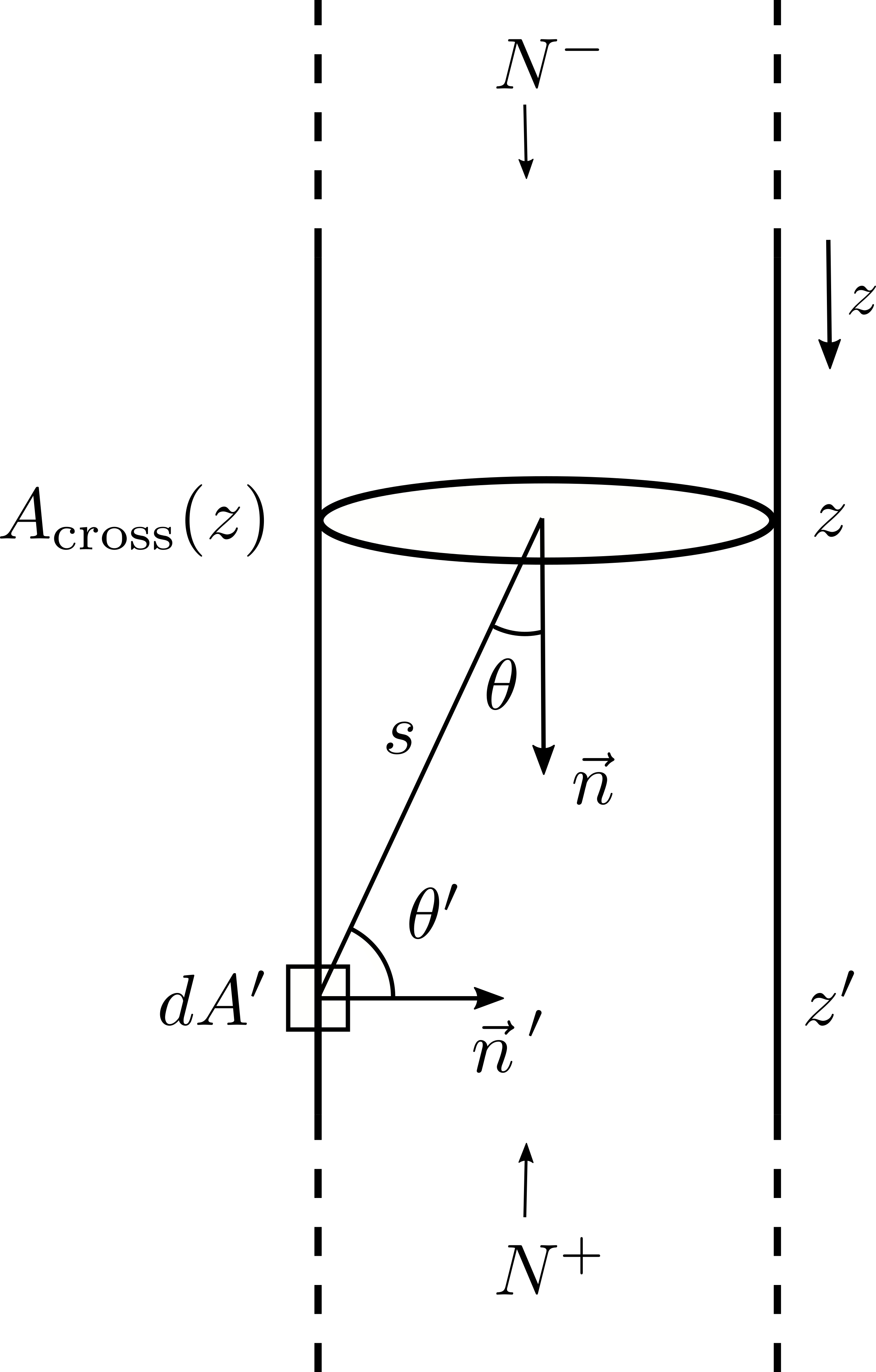
There are two key insights behind Knudsen diffusion. First, from the molecular flow hypothesis, it is assumed that the molecules crossing \(A_\mathrm {cross}(z)\) have as origin points reflections through the geometry. Therefore, the number of molecules \(dN^+\) coming from a surface element \(dA'\) and arriving at the cross-section at a distance \(s\) can be written as
\(\seteqnumber{0}{3.}{12}\)\begin{align} \label {eq::differential_number} dN^+ = (1-\beta (z'))\Gamma _\mathrm {imp}(z') \int _{A_\mathrm {cross}}\frac {\cos {\theta '}\cos {\theta }}{\pi s^2}\,dA\,dA'\, , \end{align} where \(\theta \) represents the angles between \(t\) and the surface normals. Equation (3.13) is analogous to the radiosity formulation of Eq. (2.20) without direct visibility contributions. However, instead of accumulating the flux at each surface element, it is calculated at the cross-section, which is not a part of the surface. By using the approximation \(\beta << 1\), the Hertz-Knudsen equation from Eq. (3.7), and the definition of the differential-finite view factor [98] as
\(\seteqnumber{0}{3.}{13}\)\begin{align} \label {eq::differential_finite_view_factor} F_{dA'-A} = \int _{A_\mathrm {cross}}\frac {\cos {\theta '}\cos {\theta }}{\pi s^2}\,dA\, , \end{align} then the number of incoming molecules can be written as
\(\seteqnumber{0}{3.}{14}\)\begin{align} \label {eq::incoming_molecules_view_factor} N^+ = \frac {1}{4}\overline {v}\int _z^\infty n(z') F_{dA'-A}(z'-z) dA'\, . \end{align} It is important to note that the Hertz-Knudsen equation only states a linear relationship between the concentration and the impinging flux on the surface. It is not valid for \(\Gamma _\mathrm {cross}\), since by definition it is a net flux and not an impinging flux on the container wall. The formulation in Eq. (3.15) is useful since it enables the use of standard, pre-calculated tables where the view factors are written as a function of \(z'-z\) for several geometries [107]. Attention must be placed on the correct use of the chain rule to transform the integration variable from \(dA'\) to \(dz'\) when considering any particular geometry.
To this point, the derivation has not veered far from the radiosity approach. This leads to the second key insight: To avoid the occurrence of an integral equation in \(n\) alike that in \(\Gamma _\mathrm {imp}\) in Eq. (2.20), the concentration is approximated via a Taylor expansion around \(z\), similarly to Eq. (3.9):
\(\seteqnumber{0}{3.}{15}\)\begin{align} \label {eq::concentration_taylor_z} n(z') = n(z) + (z'-z)\frac {dn}{dz} + (z'-z)^2\frac {d^2n}{dz^2} +... \end{align} Thus, after performing the change of variables \(z'-z \rightarrow z'\), Eq. (3.15) reads:
\(\seteqnumber{0}{3.}{16}\)\begin{align} \label {eq::incoming_molecules_plus} N^+ = \frac {1}{4}\overline {v} n(z)\int _0^\infty F_{dA'-A}(z') dA' + \frac {1}{4}\overline {v} \frac {dn}{dz} \int _0^\infty z' F_{dA'-A}(z') dA' +... \end{align} By analogy, the equation for \(N^-\) reads:
\(\seteqnumber{0}{3.}{17}\)\begin{align} \label {eq::incoming_molecules_minus_first} N^- = \frac {1}{4}\overline {v} n(z)\int _{-\infty }^0 F_{dA'-A}(z') dA' + \frac {1}{4}\overline {v} \frac {dn}{dz} \int _{-\infty }^0 z' F_{dA'-A}(z') dA' + ... \end{align} Most view factor tables implicitly assume a strictly positive axial distance \(z'\). However, from the interpretation of the view factor as the mutual visibility between two surfaces, it is clear that it must be symmetric in \(z'\), so the property
\(\seteqnumber{0}{3.}{18}\)\begin{align} \label {eq::view_factor_evenness} F_{dA'-A}(z') = F_{dA'-A}(-z') \end{align} must hold. This can be imposed without loss of generality by imposing the absolute value function over the odd exponents of \(z'\) on the expressions from the view factor tables [107]. Therefore, Eq. (3.18) can be simplified by reversing the integration bounds and by changing the sign of the integration variable \(z' \rightarrow -z'\):
\(\seteqnumber{0}{3.}{19}\)\begin{align} \label {eq::incoming_molecules_minus} N^- = \frac {1}{4}\overline {v} n(z)\int _0^\infty F_{dA'-A}(-z') dA' + \frac {1}{4}\overline {v} \frac {dn}{dz} \int _0^\infty (-z') F_{dA'-A}(-z') dA' + ... = \frac {1}{4}\overline {v} n(z)\int _0^\infty F_{dA'-A}(z') dA' - \frac {1}{4}\overline {v} \frac {dn}{dz} \int _0^\infty z' F_{dA'-A}(z') dA' + ... \end{align}
When combining the results of Eqs. (3.17) and (3.20) into Eq. (3.12), all terms containing the even-order terms of the Taylor expansion (\(n\), \(d^2n/dz^2\), \(...\)) cancel out. Thus, after truncating the expansion on the first-order term, the following diffusion equation is obtained
\(\seteqnumber{0}{3.}{20}\)\begin{align} \label {eq::standard_knudsen_diffusion} \Gamma _\mathrm {cross}(z) = -D_\mathrm {Kn}(z)\frac {dn}{dz}\, , \end{align} where the Knudsen diffusivity \(D_\mathrm {Kn}(z)\) for a long feature is
\(\seteqnumber{0}{3.}{21}\)\begin{align} \label {eq::standard_knudsen_diffusivity} D_\mathrm {Kn}(z) = \frac {\overline {v}}{2A_\mathrm {cross}(z)}\int _0^\infty z' F_{dA'-A}(z') dA'\, . \end{align}
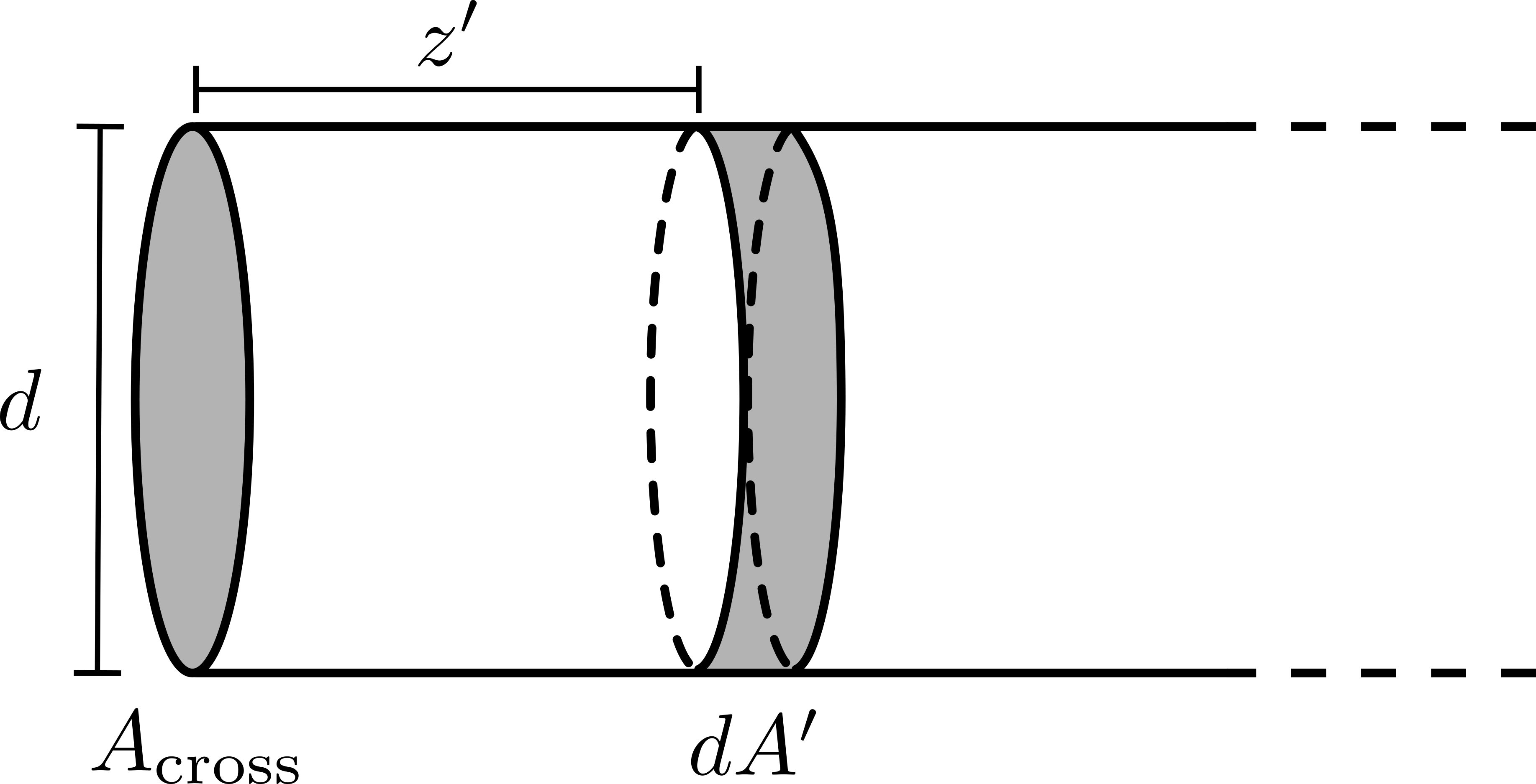
Although Eq. (3.22) still requires the calculation of an integral, it does not depend on \(n\). Therefore, it is not an integral equation. Save for the dependence on \(\overline {v}\) which can be straightforwardly calculated using Eq. (3.4), \(D_\mathrm {Kn}\) is a strictly geometric property similar to the \(W\) transmission quantity proposed by Clausing [114, 115]. As an example, the classical result of Knudsen diffusion in a long cylinder can be recovered by considering the geometry represented in Fig. 3.3.
Figure 3.3 shows the coordinate system for the calculation of the view factor inside a long cylinder between a lateral area element and a circular disk at the base, separated by the axial distance \(z'\). From the cylinder geometry, it is evident that \(A_\mathrm {cross}=\pi d^2/4\) and \(dA' = \pi d\, dz'\). The view factor in this configuration has been calculated [107, 121, 122] and takes the form
\(\seteqnumber{0}{3.}{22}\)\begin{align} \label {eq::cylinder_view_factor} F_{dA'-A}(z') = \frac {\left ( \frac {z'}{d} \right )^2 + \frac {1}{2}}{\sqrt {\left ( \frac {z'}{d} \right )^2 + 1}} - \left | \frac {z'}{d} \right |\, . \end{align} After replacing these terms in Eq. (3.22) and performing the integration, the standard result for the diffusivity is recovered:
\(\seteqnumber{0}{3.}{23}\)\begin{align} \label {eq::standard_knudsen_diffusivity_cylinder} D_\mathrm {Kn} = \frac {1}{3}\overline {v}d \end{align}
Equation (3.24) is remarkable for its clear analogy with the self-diffusion coefficient from Eq. (3.11). From an intuitive perspective, it appears as if Knudsen diffusion simply corresponds to self-diffusion after replacing the mean free path \(\lambda \) by a characteristic geometric length \(d\). However, Section 3.3 discusses issues which arise if this analogy is fully assumed at face value without a more careful consideration of the geometry.
To correctly model the reactive transport inside the feature, Eq. (3.21) is not sufficient. The intent behind the original development of the theory was to capture the flow between two reservoirs of constant pressure connected by a tube [112]. No attention is placed on the state of the surface inside this tube, particularly since the approximation of very low \(\beta \) is imposed. However, for semiconductor processing applications, the goal is to achieve an accurate description of the surface through which Knudsen transport takes place. Accordingly, a surface advection velocity function can be constructed from surface-chemical information. A fuller description of the chemical phenomena is achieved by imposing conservation of mass in the presence adsorption losses at the sidewalls [50, 123]:
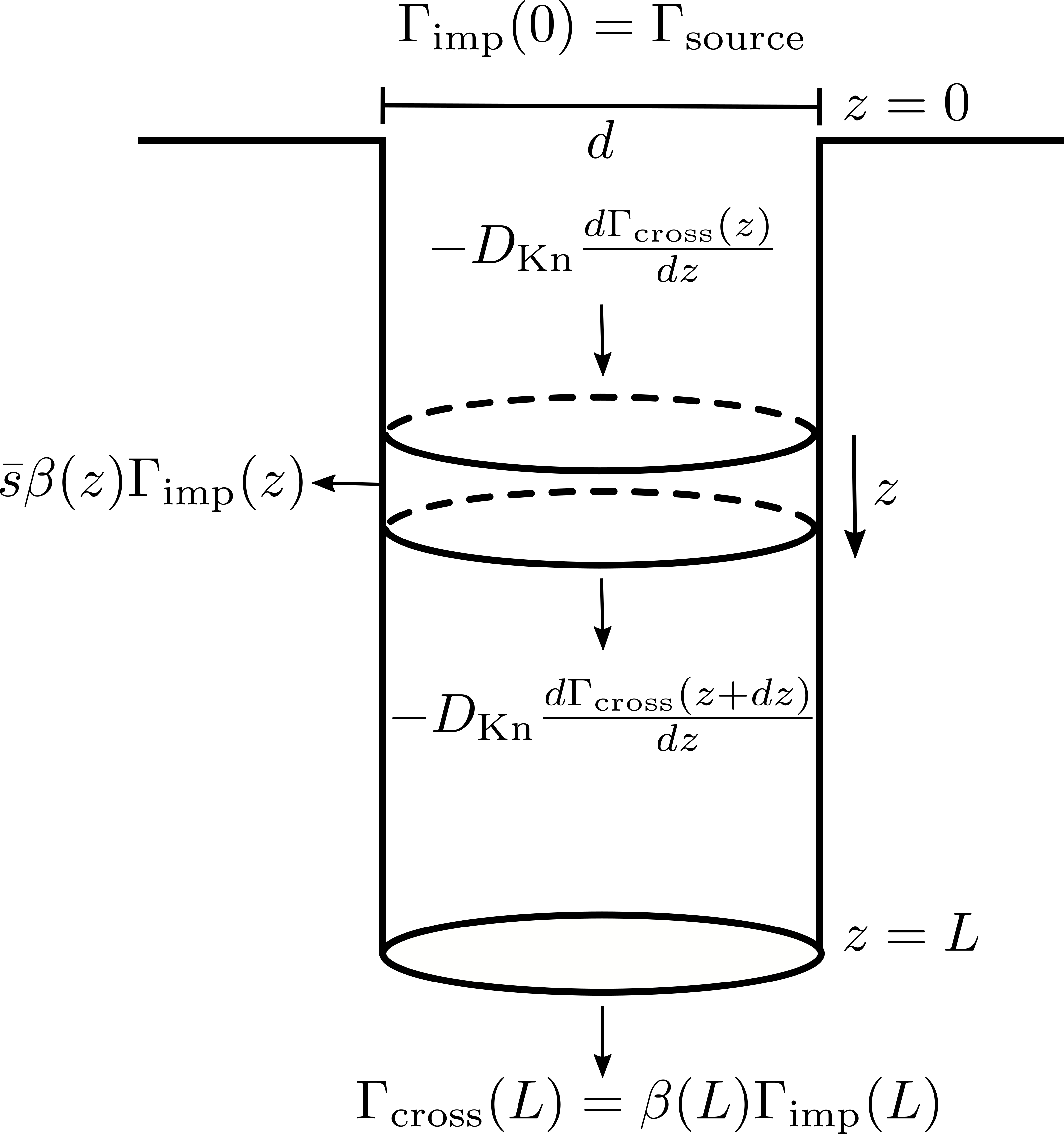
\(\seteqnumber{0}{3.}{24}\)\begin{align} \label {eq::consevation_mass} \frac {\partial n(z,t)}{\partial t}+\frac {\partial \Gamma _\mathrm {cross}(z,t)}{\partial z} = -\overline {s}\beta (z)\Gamma _\mathrm {imp}(z) \end{align} From the discussion in Section 2.2, it is usually assumed that transport equilibrates much more quickly than the surface kinetics. This is also named the frozen surface approximation [124], and it means that the first term in Eq. (3.25) is zero (i.e., a steady-state condition in \(n\)), even if the surface kinetics have not equilibrated (\(d\Theta /dt \neq 0\)). This steady-state conservation of mass is illustrated in Fig. 3.4. The right-hand side of Eq. (3.25) represents the volumetric losses due to adsorption, where \(\overline {s}\) is the specific surface area, i.e., the surface area per unit volume. For a cylinder, \(\overline {s} = 4/d\).
After replacing the previously calculated results for a cylinder and the Hertz-Knudsen Eq. (3.7) into Eq. (3.25), the following ordinary differential equation (ODE) is obtained:
\(\seteqnumber{0}{3.}{25}\)\begin{align} \label {eq::concentration_ODE} -D_\mathrm {kn}\frac {d^2n}{dz^2} = -\overline {s}\beta (z)\Gamma _\mathrm {imp}(z) \implies \frac {1}{3}\overline {v}d \, \frac {d^2n}{dz^2} = \frac {4}{d}\beta (z)\frac {1}{4}\overline {v}n(z) \end{align} This equation can be further simplified by assuming constant \(\beta \) and by performing the change of variables \(z \rightarrow \varepsilon L\), with \(L\) being the length of the cylinder. Then,
\(\seteqnumber{0}{3.}{26}\)\begin{align} \label {eq::thiele_modulus_ODE} \frac {d^2n}{d\varepsilon ^2} = 3\beta \frac {L^2}{d^2} n(\varepsilon ) = h_T^2 \, n(\varepsilon )\, , \end{align} where \(h_T^2\) is the Thiele modulus, also called the second Damköhler number [50, 124], which is the ratio of the reaction rate to the transport rate. By identifying the AR from Eq. (2.19), \(h_T^2\) takes the form
\(\seteqnumber{0}{3.}{27}\)\begin{align} \label {eq::thiele_modulus} h_T^2 = 3\beta (\mathrm {AR})^2\, . \end{align}
For many semiconductor processing techniques, the goal is to achieve conformality, that is, a uniform distribution of growth or etch rates throughout the geometry. From Eq. (3.27), this means having a value \(h_T^2 <<1\). A dimensionality analysis in Eq. (3.28) exposes the challenge of achieving good conformality in high AR structures. There is a quadratic dependence on the AR which can only be combatted with linear improvements in \(\beta \). The issue of non-ideal conformality in atomic layer processing (ALP) is the subject of Chapter 4.
Equation (3.26) is an ODE of the second degree. Therefore, it requires two boundary conditions (BCs). First, as discussed in Section 2.3, it is always assumed that there is a constant distribution of reactants in the region of the reactor neighboring the feature, i.e., the source plane, which for a long feature is defined as the plane \(z{=}0\) at the top. This means that the reactor is efficient enough to maintain a constant impinging flux \(\Gamma _\mathrm {imp}(z{=}0) {=} \Gamma _\mathrm {source}\). In the context of the Hertz-Knudsen equation, this is equivalent to maintaining a constant concentration (\(n_0\)) at the top:
\(\seteqnumber{0}{3.}{28}\)\begin{align} \label {eq::first_BC} n(0) = n_0 \end{align} The second BC is defined at the bottom (\(z{=}L\)). This BC must also have a different treatment than in the classical case of a tube connecting two reservoirs with fixed pressures. This situation would yield a BC similar to Eq. (3.29). Instead, the BC at \(z{=}L\) is that the flux must match the losses due to adsorption, thus preserving the mass balance. This is achieved through a Robin BC which takes the form [30]:
\(\seteqnumber{0}{3.}{29}\)\begin{align} \label {eq::second_BC} \Gamma _\mathrm {cross} (L) = \beta (L)\Gamma _\mathrm {imp}(L) \implies -D_\mathrm {Kn} \left . \frac {dn}{dz} \right |_{z=L} = \beta (L)\frac {1}{4}\overline {v}n(L) \end{align}
Under the approximation of constant \(\beta \) and the aforementioned BCs, the ODE from Eq. (3.26) has an exact solution [50] which can be written in terms of the normalized flux normalization \(\hat {\Gamma }_\mathrm {imp}(z)\) following the convention from Eq. (2.7):
\(\seteqnumber{0}{3.}{30}\)\begin{align} \label {eq::solution_constant_sticking} \hat {\Gamma }_\mathrm {imp}(z) = \frac {\Gamma _\mathrm {imp}(z)}{\Gamma _\mathrm {source}} = \frac {n(z)}{n_0} = \frac { 3 \sqrt {\beta } \sinh \left (\frac {\sqrt {3\beta } (L-z)}{d}\right )+4 \sqrt {3} \cosh \left (\frac {\sqrt {3\beta } (L-z)}{d}\right )}{3 \sqrt {\beta } \sinh \left (\frac {\sqrt {3\beta } L}{d}\right )+4 \sqrt {3} \cosh \left (\frac {\sqrt {3\beta } L}{d}\right )} \end{align}