Chapter 2 Review of Reactive Transport Models for Topography Simulation
The ultimate goal of topography simulation is to guide the development of semiconductor devices through a physically realistic description of structures after etching and deposition. To achieve this goal, an accurate topography
simulation must possess two fundamental characteristics: A method for robustly representing the advecting surfaces and realistic models describing the local surface speeds stemming from the complex reactive transport of the
involved reactants. This chapter presents a review of these reactive transport models including their context within topography simulation.
Firstly, a short overview of the chosen method for surface advection, the level-set (LS) method, is presented. Particular attention is placed on the term linking the topography simulation with reactive transport modeling: The
velocity field \(v(\vec {r},t)\). Afterward, a review of Langmuir adsorption kinetics is given which is necessary for connecting the particle fluxes with the local surface state. Finally, an overview of the explored approaches to
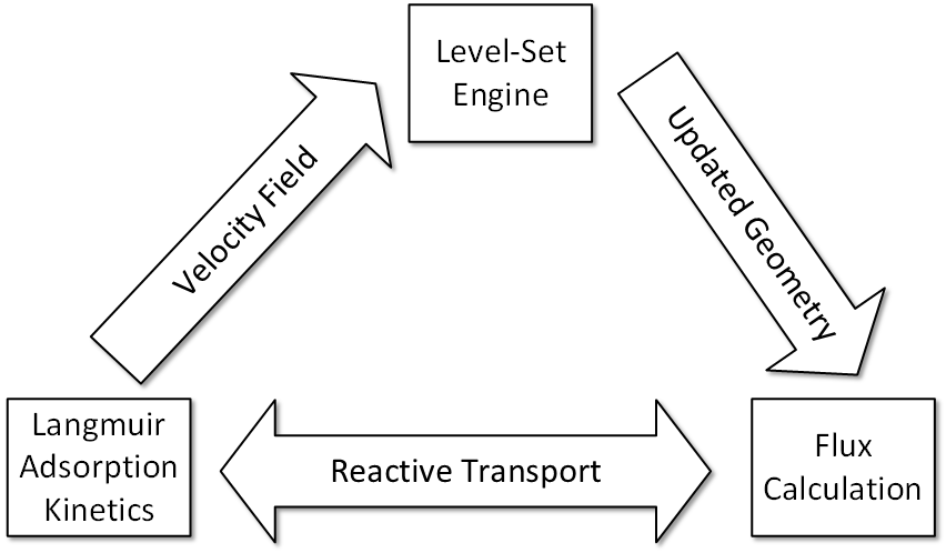
calculate the local particle fluxes is provided. Importantly, the flux calculation and the chemical state of the surface might mutually interact which is the source of complex reactive transport behavior. The interplay of these
elements in one iteration cycle of the topography simulation is visually represented in Fig. 2.1. The evaluation and application of reactive transport models to specific etching
and deposition problems is discussed in subsequent chapters of this dissertation.
Figure 2.1: Flowchart depicting one iteration cycle of an LS based topography simulation. The two-headed arrow linking the flux calculation to Langmuir adsorption kinetics indicates their mutual dependence in the calculation of
the reactive transport.
2.1 The Level-Set Method
The fundamental challenge of surface advection algorithms in semiconductor manufacturing is that the involved surfaces undergo very complex processes [41]. In particular, the surfaces can undergo changes in topology, such
as the complete perforation of a material layer after an etch step, which make explicit surface representations exceedingly difficult [42]. Although cell-based representations can also handle such topological changes [52],
they lack sufficient information about the surface position and are thus inaccurate in their calculations, e.g., curvatures and normals [42, 53].
Thus, the accurate LS method has emerged as a standard in topography simulation for process technology computer-aided design (TCAD). It is widely implemented in commercial simulators, such as Synopsys’ Sentaurus
Topography [54], Silvaco’s Victory Process [55], and the Florida object-oriented multipurpose simulator (FLOOXS) [29, 56], as well as open-source tools like ViennaTS [57].
The LS method is based on an implicit surface representation. Unlike explicit representations, where surface points and connecting elements are directly stored, in this implicit representation a function \(\phi (\vec {r},t)\) is
defined for all points in the domain. In the LS method [58, 59], the surface \(S\) bounding a volume \(V\) is recovered from the property \(\phi (\vec {r},t) = 0\) for all points on \(S\). That is, \(S\) is described by the
zero level-set of \(\phi (\vec {r},t)\), as long as \(\phi (\vec {r},t) > 0\) on the outside of \(V\) and \(\phi (\vec {r},t) < 0\) on its inside. A common choice of \(\phi (\vec {r},t)\) for describing surfaces
resulting from semiconductor processing [60, 61] is that of the signed-distance function (SDF), that is, the distance \(d\) between \(\vec {r}\) and \(S\) with the necessary sign:
The evolution of the surface described in Eq. (2.1) is driven by a velocity field \(\vec {v}(\vec {r},t)\). The following Hamilton-Jacobi equation can then be
derived for the evolution of the surface [58, 62]:
To obtain a numerical solution, Eq. (2.2) is conventionally discretized on a regular rectangular grid with spacing \(\Delta x\). The involved partial derivatives are
then approximated using finite difference schemes [63]. Additionally, it should be remarked that there is a difference between fast marching and narrow band LS methods [42]. In the former, the values
of \(\phi (\vec {r},t)\) are stored in the entire domain, thus requiring the fast marching method to propagate the values from the interface [64], whereas in the latter only values near the surface are stored [65].
Both methods have found application (e.g., fast marching and narrow band respectively in Silvaco’s Victory Process [55] and ViennaTS [57]) and are used in this dissertation. Although developments in fast marching
methods are an area of activity for researchers of the Christian Doppler Laboratory for High Performance TCAD [66, 67], a more detailed description is outside the scope of the presented research.
Instead, the principal focus of this dissertation is the study of phenomenological methods for the construction of the term \(v(\vec {r},t)\). For a reactive transport model to be useful for topography simulations, it should
ultimately generate a velocity field, i.e., etch or growth rates must be determined for the whole surface. It is noteworthy that, for the method described by Eq. (2.2), only the normal component \(v(\vec {r},t)\) of the proper velocity field \(\vec {v}(\vec {r},t)\) is necessary. Therefore, it would be more accurate to describe \(v(\vec {r},t)\)
as a speed field. However, for consistency with the established literature, this dissertation will hitherto refer to \(v(\vec {r},t)\) as the velocity field. When the involved process results in material deposition, the
convention is that \(v(\vec {r},t)\) carries a positive sign. Then, \(v(\vec {r},t)\) can also be denoted as the growth rate \(\textit {GR}(\vec {r},t) = v(\vec {r},t)\). Etching processes result in an etch rate with a
negative sign, i.e., the etch rate \(\textit {ER}(\vec {r},t) = -v(\vec {r},t)\).