Phenomenological Single-Particle
Modeling of Reactive Transport
in Semiconductor Processing

2.3 Approaches to Calculate Local Fluxes

In Section 2.2, all terms of Langmuir adsorption kinetics in Eq. (2.3) are discussed except for the local impinging particle flux ${\mathrm{\Gamma }}_{\mathrm{imp}}(\overrightarrow{r})$. Its calculation is the focus of this section, where four classes of methods are presented: Constant flux, bottom-up visibility calculation, top-down pseudo-particle tracking, and one-dimensional (1D) models. In particular, the relationship mediated by the coverage-dependent reflection given by Eq. (2.4) between the local fluxes and the surface state is explored, including required approximations.

At the heart of these flux calculation approaches are considerations of the flow regime. This analysis requires defining two characteristic lengths of the transport processes: The mean free path $\lambda$, given by the probability of particle-particle collisions; and a representative length of the geometry $d$, e.g., the diameter if the geometry is a cylinder. From those, the Knudsen number can be constructed as [30]:

$$\begin{array}{}\text{(2.6)}& \text{Kn}=\frac{\lambda }{d}.\end{array}$$ $\text{Kn}$ is a measure of the relative probability of a particle-particle collision to a particle-geometry collision. Therefore, the molecular flow regime is achieved for high Knudsen numbers, typically assumed to be $\text{Kn}>10$ [80], i.e., a collision with the geometry is at least ten times more likely than that with another particle. Many semiconductor processing techniques, particularly those involving gas- or plasma-phase, occur in a high vacuum chamber and thus in the molecular flow regime. Therefore, this regime is conventionally assumed for the flux calculation, although allowances for the transitional flow regime (${10}^{-1}<\text{Kn}<10$) are discussed for the top-down and 1D approaches.

All calculation methods of ${\mathrm{\Gamma }}_{\mathrm{imp}}(\overrightarrow{r})$ require a reference flux value ${\mathrm{\Gamma }}_{\mathrm{source}}$ which is the reactant flux at an imaginary boundary between the feature-scale and the reactor-scale called the source plane. Although ${\mathrm{\Gamma }}_{\mathrm{source}}$ can be experimentally inferred [43] or calculated with detailed reactor models [38, 81], another approach is to normalize the impinging flux to the source flux, i.e.,

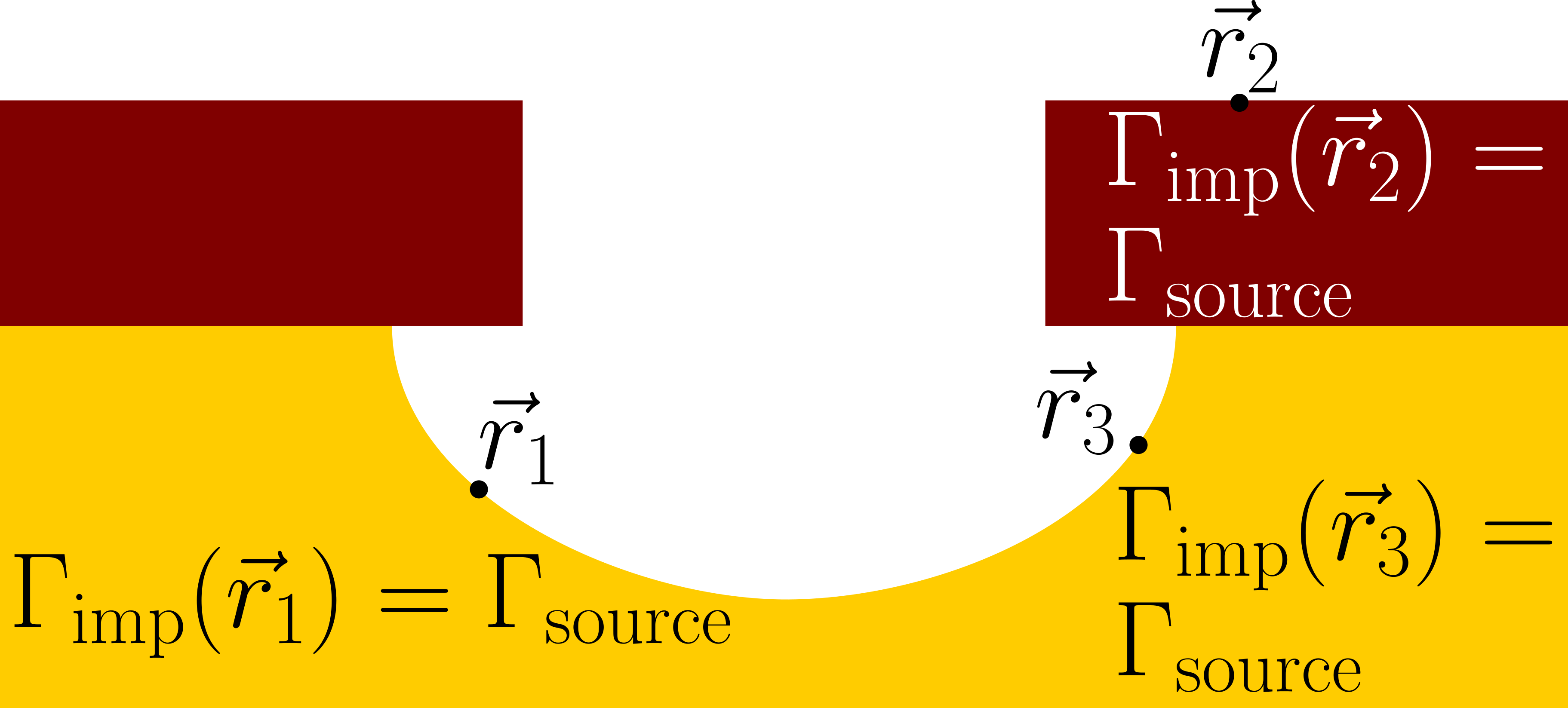
$$\begin{array}{}\text{(2.7)}& {\hat{\mathrm{\Gamma }}}_{\mathrm{imp}}(\overrightarrow{r})=\frac{{\mathrm{\Gamma }}_{\mathrm{imp}}(\overrightarrow{r})}{{\mathrm{\Gamma }}_{\mathrm{source}}}.\end{array}$$ This is viable since ${\mathrm{\Gamma }}_{\mathrm{source}}$ is also, by definition, the local flux received by a fully visible surface site (c.f. point ${\overrightarrow{r}}_2$ in Fig. 2.5). Therefore, instead of performing a complex calculation of ${\mathrm{\Gamma }}_{\mathrm{source}}$, ${\hat{\mathrm{\Gamma }}}_{\mathrm{imp}}(\overrightarrow{r})$ is calculated in its normalized form directly. Then, rather than relying on a complex formula such as Eq. (2.5), the velocity field can be calculated from the (etch or deposition) plane wafer rate $\mathit{PWR}$. An example of such field is

$$\begin{array}{}\text{(2.8)}& v(\overrightarrow{r},t)={\hat{\mathrm{\Gamma }}}_{\mathrm{imp}}(\overrightarrow{r},t)\cdot \mathit{PWR}\end{array}$$ which can be advantageous since the $\mathit{PWR}$ can be straightforwardly related to experimental measurements. For instance, lithography masks often include a large exposed test structure which is expected to receive the maximum amount of reactants ${\hat{\mathrm{\Gamma }}}_{\mathrm{imp}}=1$ and be etched with the $\mathit{PWR}$.

Lastly, it is noteworthy that the incoming flux might be characterized not only by its magnitude but also by an angular and energy distribution, particularly when ion acceleration due to plasma interactions are involved. The bottom-up and top-down methods, as discussed below, can take these distributions into account for the local flux calculations. However, the focus of this dissertation is the study of thermal processes, that is, those where there is no preferential incoming or reflection direction.
Nonetheless, Eq. (2.7) is always valid if ${\mathrm{\Gamma }}_{\mathrm{source}}$ is interpreted as the absolute value of the flux, since a fully visible element will always receive ${\mathrm{\Gamma }}_{\mathrm{source}}$ regardless of the source angular and energy distribution.

2.3.1 Constant Flux

The most straightforward approach for the reactive transport calculation is the constant flux approximation, illustrated in Fig. 2.2. In this approach, all exposed surface elements receive the same ${\mathrm{\Gamma }}_{\mathrm{source}}$, thus the velocity field is strictly a function of local material properties. Although simple, this method still requires some computational effort since only the exposed surfaces must be detected, disregarding, e.g., eventual voids [82, 83].

This apparent simplicity can obfuscate the deeper physical assumptions necessary for the application of this reactive transport approach. One situation which enables this approach is the surface-controlled regime [84], which is commonly observed in anisotropic wet etching [85, 86]. In it, there must be a large enough availability of reactants such that all exposed surface sites become fully saturated. Thus, according to Eq. (2.4), the sticking coefficient approaches zero ($\beta \to 0^{+}$). Additionally, any local depletion due to the ongoing surface-chemical reactions is immediately replenished by transported reactants. Thus, any anisotropy is strictly due to local surface-controlled phenomena and the constant flux approach holds.

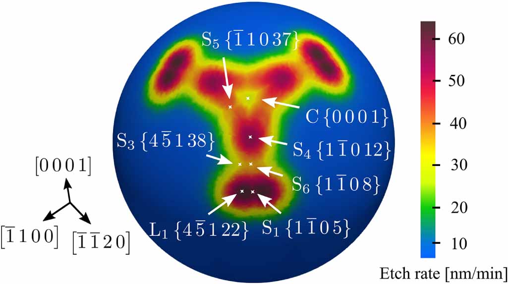
Accordingly, the velocity field is constructed with strictly local parameters. For anisotropic wet etching, the most common surface-controlled phenomenon is the crystallographic orientation dependence of the etch rate [85]. Thus, the velocities are a function of the surface normal $\overrightarrow{n}$, and the anisotropy is only due to local surface properties, notably $\overrightarrow{n}$, and not due to differences in flux, as long as the surface-controlled regime is experimentally maintained. One approach for determining this locally-varying velocity field for crystallographic orientation-dependent phenomena, proposed by Toifl et al. [87], involves interpolating between the crystal directions ${\overrightarrow{m}}_i$

$$\begin{array}{}\text{(2.9)}& v(\overrightarrow{n})=v_0+\sum _i{\alpha }_i⟨\overrightarrow{n},{\overrightarrow{m}}_i{⟩}^{{\omega }_i}H(⟨\overrightarrow{n},{\overrightarrow{m}}_i⟩).\end{array}$$

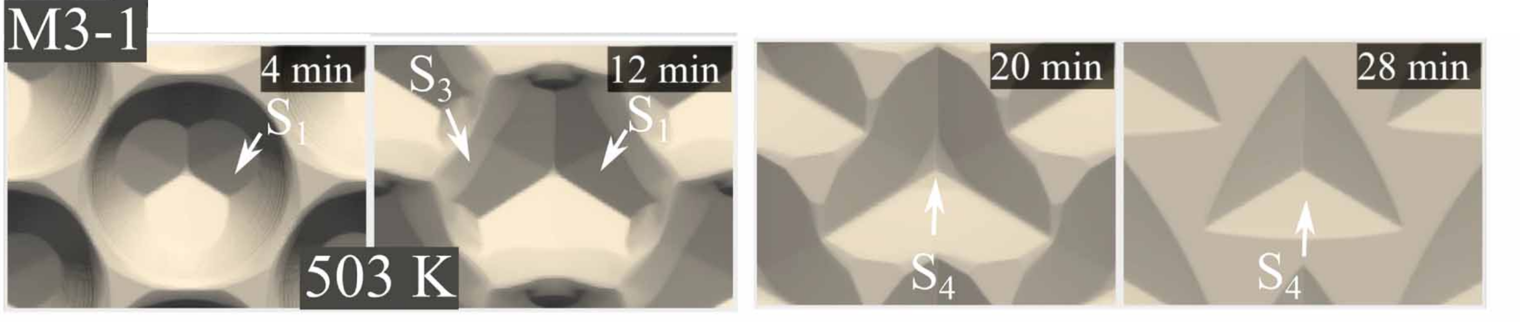
In Eq. (2.9), $H$ is the Heaviside function, $⟨\cdot ,\cdot ⟩$ is the inner product, $v_0$ is the isotropic component of the velocity field, and ${\alpha }_i$ and ${\omega }_i$ are parameters which can be constructed from considering the etch rates in the ${\overrightarrow{m}}_i$ directions. An example of Eq. (2.9), parameterized to the etching of sapphire from a mixture of sulfuric acid to phosphoric acid on a 3:1 ratio (M3-1) at 503 K, is shown in Fig. 2.3. The effect of applying this velocity field to an array of cones is shown in Fig. 2.4, highlighting the strong profile variation strictly due to local properties.

However, surface saturation is not the only condition in which the constant flux approximation is valid. In isotropic wet etching, it is commonly necessary to establish the transport-controlled regime, where the etching is limited by rate of reactant transport. Otherwise, an oversupply of reactants can lead to more complex surface phenomena and, thus, undesired anisotropy [84]. Therefore, there is a trade-off which must be carefully balanced to achieve true isotropy: Excessive reactant supply can lead to anisotropy from surface reactions, while insufficient supply can lead to anisotropy due to a gradient in the flux distribution.

Therefore, achieving a truly isotropic wet etching process, wherein the constant flux approximation must necessarily hold, is fairly complex. Either a surface-controlled reaction with no spurious anisotropic component or a finely-balanced transport-controlled regime must be constructed. However, if this is achieved, the topography simulation becomes somewhat trivial, and the velocity field can be expressed as

$$\begin{array}{}\text{(2.10)}& v(\overrightarrow{r},t)={\mathit{\text{ER}}}_{\mathrm{material}},\end{array}$$ where ${\mathit{\text{ER}}}_{\mathrm{material}}$ represents the measurable isotropic etch rate of an exposed material.

2.3.2 Bottom-Up Visibility Calculation

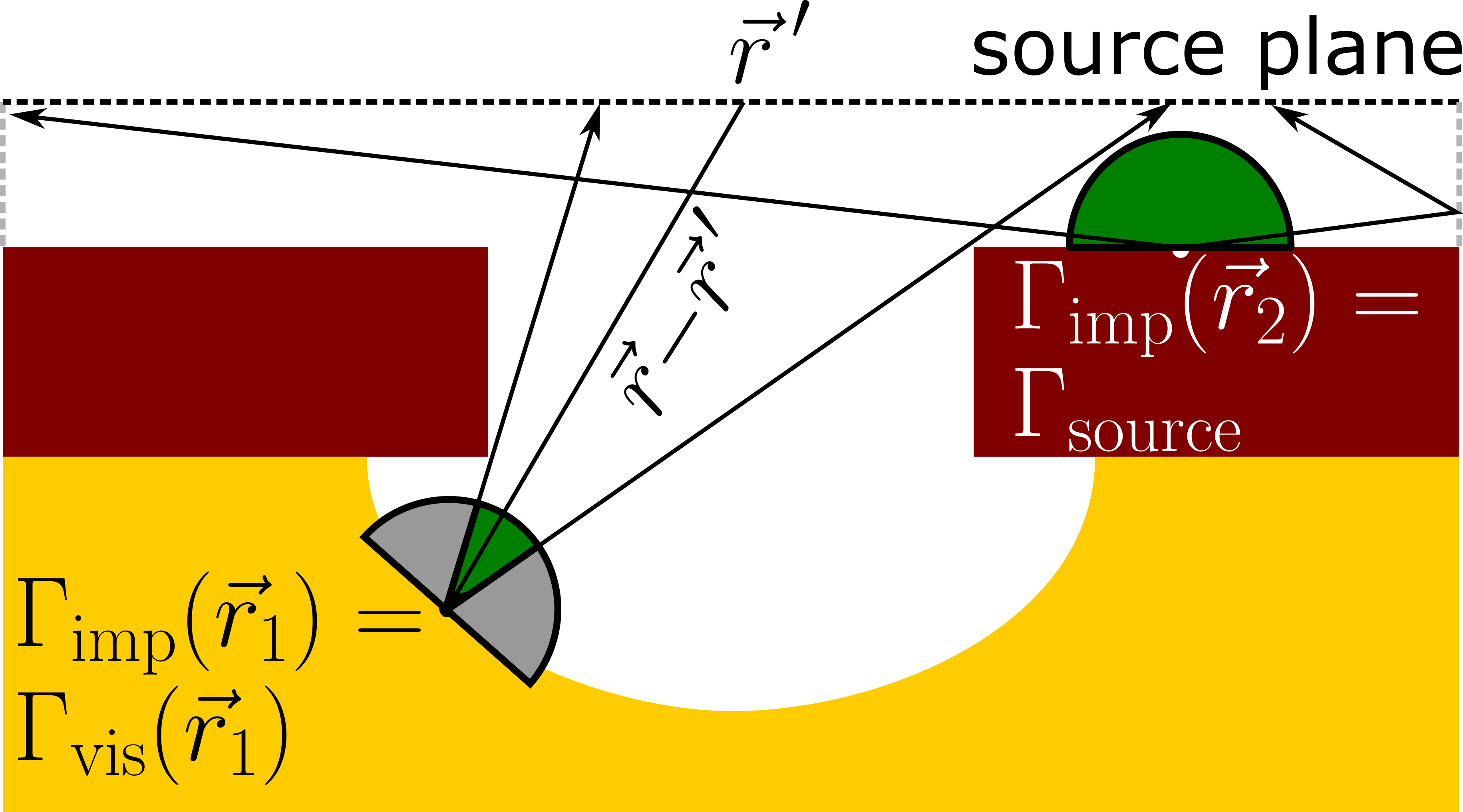
Moving beyond the straightforward constant flux approach, the bottom-up calculation adds nuance to the reactive transport by incorporating visibility effects. This is represented in Fig. 2.5, where a fully visible surface element (${\overrightarrow{r}}_2$) still receives ${\mathrm{\Gamma }}_{\mathrm{source}}$, while a partially obstructed element (${\overrightarrow{r}}_1$) receives a smaller flux due to reduced visibility ${\mathrm{\Gamma }}_{\mathrm{vis}}$. Importantly, visibility is here defined as a continuous variable between $0$ and ${\mathrm{\Gamma }}_{\mathrm{source}}$, while exposure, as defined in Section 2.3.1, is strictly binary. Thus, the visibility-dependent flux can be stated as an integral over the entire source plane [61]

$$\begin{array}{}\text{(2.11)}& {\mathrm{\Gamma }}_{\mathrm{vis}}(\overrightarrow{r})={\int }_{\mathrm{source}}{\mathrm{\Gamma }}_{\mathrm{source}}(\overrightarrow{r}-{\overrightarrow{r}}^{\prime })⟨\overrightarrow{n},{\overrightarrow{n}}^{\prime }⟩d{\overrightarrow{r}}^{\prime },\end{array}$$ where $\overrightarrow{r}$ and $\overrightarrow{n}$ are the position and unit normal vector of the point where the flux is evaluated, respectively; and ${\overrightarrow{r}}^{\prime }$ and ${\overrightarrow{n}}^{\prime }$ are the positions and normals at the source plane over which the integral iterates. Since the flux calculation is performed at each surface element independently, this method is denoted as bottom-up.

In Eq. (2.11), the source flux has an angular dependence on the outgoing direction $\overrightarrow{r}-{\overrightarrow{r}}^{\prime }$, thus ${\mathrm{\Gamma }}_{\mathrm{source}}(\overrightarrow{r}-{\overrightarrow{r}}^{\prime })$ must be constructed attentively so that the total integral is correctly normalized. An isotropic source flux distribution has to follow a cosine distribution, i.e. [89]

$$\begin{array}{}\text{(2.12)}& {\mathrm{\Gamma }}_{\mathrm{source},\mathrm{isotropic}}(\overrightarrow{r}-{\overrightarrow{r}}^{\prime })={\mathrm{\Gamma }}_{\mathrm{source}}\frac{1}{\pi }\frac{⟨(\overrightarrow{r}-{\overrightarrow{r}}^{\prime }),{\overrightarrow{n}}^{\prime }⟩}{||\overrightarrow{r}-{\overrightarrow{r}}^{\prime }||},\end{array}$$ so that a fully visible surface element receives a flux with magnitude ${\mathrm{\Gamma }}_{\mathrm{source}}$. Additionally, Eq. (2.11) enables more complex source flux distributions such as those more vertically focused due to plasma-accelerated ions which can be modeled with a $\kappa$-power cosine distribution

$$\begin{array}{}\text{(2.13)}& {\mathrm{\Gamma }}_{\mathrm{source},\mathrm{focused}}(\overrightarrow{r}-{\overrightarrow{r}}^{\prime })={\mathrm{\Gamma }}_{\mathrm{source}}\frac{\kappa +1}{2\pi }\frac{⟨(\overrightarrow{r}-{\overrightarrow{r}}^{\prime }),{\overrightarrow{n}}^{\prime }{⟩}^{\kappa }}{||\overrightarrow{r}-{\overrightarrow{r}}^{\prime }||}.\end{array}$$

The largest challenge imposed by Eq. (2.11) is the solution of the involved integral. Nonetheless, the lack of reflections greatly simplifies this challenge, since each surface position $\overrightarrow{r}$ only requires computing the contributions by the ${\overrightarrow{r}}^{\prime }$ positions on the source plane which has a constant and comparatively small number of elements.
Thus, this integral can be directly solved on the LS grid if a function which determines if $\overrightarrow{r}$ and ${\overrightarrow{r}}^{\prime }$ are mutually exposed is available [82, 90]. More recently, ray-tracing schemes have been developed by discretizing the hemisphere above each $\overrightarrow{r}$ and querying for intersections with the source plane. For example, efficient ray-tracing kernels can be used by extracting explicit meshes from the LS grid [91]. Additional performance improvements have been achieved by adaptive sampling of the hemisphere [92] and by restricting the number of surface elements wherein the flux is calculated [93].

This bottom-up approach has critical implications for the reactive transport modeling. As previously stated, Eq. (2.11) does not include reflections, therefore, it can only model processes with $\beta =1$. This puts the bottom-up visibility calculation in stark contrast to the constant flux approach which captures processes with near-zero sticking coefficient. Thus, these two approaches can be understood as the two extremes of reactive transport with constant sticking coefficient. There are several physical processes which are commonly modeled with a sticking coefficient of unity, most notably physical vapor deposition (PVD). In this category of processing techniques, the material to be deposited is vaporized and transported to the feature, where it physically interacts (i.e., without changes in its chemical composition) and forms a film [32]. If these interactions are energetically favored and occur with high efficiency without re-sputtering, then they can be adequately modeled with $\beta =1$ [30, 94]. However, more complex phenomena in PVD such as grain boundary formation, might require different values of $\beta$ [51].

To overcome this limitation on $\beta$, it is possible to reformulate Eq. (2.11) to include not only the direct visibility contributions, but also the effect of the indirect flux ${\mathrm{\Gamma }}_{\mathrm{ind}}$ reflected by the entire geometry onto $\overrightarrow{r}$ as [90]

$$\begin{array}{}\text{(2.14)}& {\mathrm{\Gamma }}_{\mathrm{imp}}(\overrightarrow{r})={\mathrm{\Gamma }}_{\mathrm{vis}}(\overrightarrow{r})+{\mathrm{\Gamma }}_{\mathrm{ind}}(\overrightarrow{r})=\beta (\overrightarrow{r}){\int }_{\mathrm{source}}{\mathrm{\Gamma }}_{\mathrm{source}}(\overrightarrow{r}-{\overrightarrow{r}}^{\prime })⟨\overrightarrow{n},{\overrightarrow{n}}^{\prime }⟩d{\overrightarrow{r}}^{\prime }+{\int }_{\mathrm{geometry}}(1-\beta ({\overrightarrow{r}}^{\prime })){\mathrm{\Gamma }}_{\mathrm{refl}}(\overrightarrow{r},{\overrightarrow{r}}^{\prime })⟨\overrightarrow{n},{\overrightarrow{n}}^{\prime }⟩d{\overrightarrow{r}}^{\prime },\end{array}$$ where ${\mathrm{\Gamma }}_{\mathrm{refl}}$ is the reflected flux which is naturally itself a function of the impinging flux at ${\overrightarrow{r}}^{\prime }$. That is, for each $\overrightarrow{r}$, the integration variable ${\overrightarrow{r}}^{\prime }$ iterates not only over the source plane but also over the surface. Thus, Eq. (2.14) is a true integral equation, since the local impinging flux depends on the distribution ${\mathrm{\Gamma }}_{\mathrm{imp}}$ over the entire geometry. This equation is exceedingly challenging to solve, since it scales with the square of the number of surface sites, as each site must compute the contributions of the whole geometry. It can be solved for arbitrary source and reflection distribution functions iteratively over multiple bounces [41]. More commonly, Eq. (2.14) is solved under the stricter approximations of constant $\beta$ and isotropic source and reflection distributions, in what is often named a radiosity approach [90, 95, 96, 97], discussed in more detail in Section 2.3.4. Nonetheless, the quadratic dependence on the number of surface elements imposes stringent performance limitations to this approach even on state-of-the-art computing systems, since the entire radiosity matrix must be calculated, stored and inverted.

2.3.3 Top-Down Pseudo-Particle Tracking

As discussed in the previous sections, the constant flux approach is valid in the $\beta \to 0^{+}$ regime. Furthermore, the bottom-up visibility calculation straightforwardly captures $\beta =1$. It is thus patently necessary to introduce a method which is able to capture reactive transport for intermediate values of $\beta$, as well as more complex physical phenomena beyond the constant sticking coefficient approximation. Although Eq. (2.14) condenses the involved physical and chemical phenomena, its direct solution is untenable for the general case due to the computational complexity of the integral equation.

Therefore, a more computationally efficient approach is the Monte Carlo tracking of pseudo-particles sampling of this integral equation, as illustrated in Fig. 2.6. These pseudo-particles are named as such because they should only be interpreted as discrete samples of the continuum integral equation. They are not representations of individual particles, e.g., chemical reactants or ions, and are, therefore, unable to capture molecular-scale phenomena. This Monte Carlo method equally splits the product of ${\mathrm{\Gamma }}_{\mathrm{source}}$ and the source plane area $A_{\mathrm{source}}$ (i.e., the total power, in analogy to radiative heat transfer [98]) among $N_{\mathrm{part}}$ pseudo-particles to achieve an initial per-pseudo-particle flux payload [89]

$$\begin{array}{}\text{(2.15)}& {\mathrm{\Gamma }}_{\mathrm{part},\mathrm{initial}}=\frac{A_{\mathrm{source}}}{N_{\mathrm{part}}}{\mathrm{\Gamma }}_{\mathrm{source}}.\end{array}$$

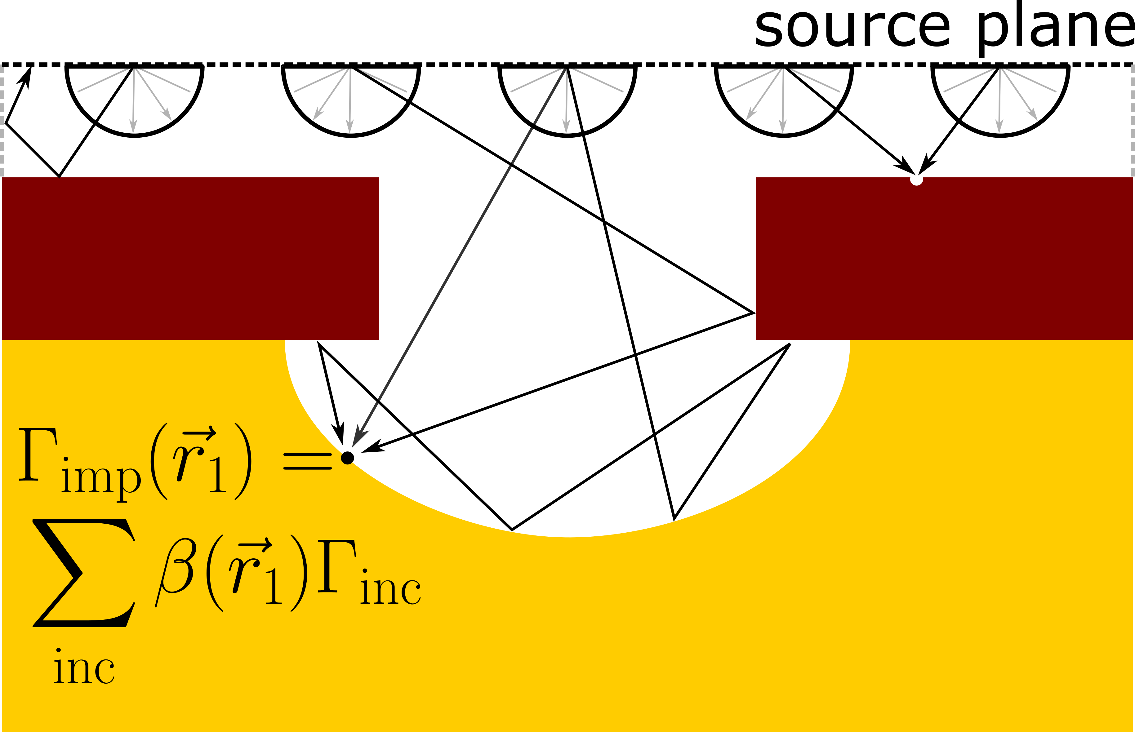
The pseudo-particles are then initialized with a uniform initial position in the source plane and an initial direction $\overrightarrow{t}$ sampled from the ${\mathrm{\Gamma }}_{\mathrm{source}}(\overrightarrow{t})$ distribution, e.g., Eq. (2.12) or Eq. (2.13) with $\overrightarrow{t}=\overrightarrow{r}-{\overrightarrow{r}}^{\prime }$. Each pseudo-particle is traced top-down through the simulation domain until it interacts with the geometry and terminates. Then, the pseudo-particle deposits its flux payload mediated by the local value of $\beta$ [41, 89, 99]. Therefore, each surface element accumulates its impinging flux as the sum over all incident pseudo-particles, each carrying its own payload ${\mathrm{\Gamma }}_{\mathrm{inc}}$

$$\begin{array}{}\text{(2.16)}& {\mathrm{\Gamma }}_{\mathrm{imp}}(\overrightarrow{r})=\sum _{\mathrm{inc}}\beta (\overrightarrow{r}){\mathrm{\Gamma }}_{\mathrm{inc}}.\end{array}$$ This formulation enables directly representing the effects of reactant reflections by generating new pseudo-particles according to a reflection distribution. These reflected pseudo-particle have their flux payload ${\mathrm{\Gamma }}_{\mathrm{refl}}$ reduced with respect to the incident pseudo-particle according to

$$\begin{array}{}\text{(2.17)}& {\mathrm{\Gamma }}_{\mathrm{refl}}=(1-\beta (\overrightarrow{r})){\mathrm{\Gamma }}_{\mathrm{inc}}.\end{array}$$ The new pseudo-particles have their initial direction sampled from the hemisphere aligned with the local normal direction. This sampling can take several forms depending on the involved physical and chemical reactions. It is usually assumed that pseudo-particles representing neutral species immediately thermalize and reflect isotropically, sampling the hemisphere with a cosine distribution similar to Eq. (2.12). However, accelerated ions can reflect specularly under certain conditions, thus requiring a distribution function depending on the incoming ray direction $\overrightarrow{t}$ [44, 75]. This process of termination and generation repeats until the pseudo-particle leaves the simulation domain or its payload drops below a threshold.

An initial approximation to be made to the top-down approach is assuming constant sticking coefficient, similarly to the discussion in Section 2.3.1 and Section 2.3.2. However, in contrast to the constant flux and bottom-up approaches, $\beta$ can now take any fixed value between the respective extremes of $0$ and $1$, including having different values for each involved material. In general, $\beta$ as described in Eqs. (2.16) and (2.17) is an arbitrary function of the position $\overrightarrow{r}$, usually depending on the local surface coverage $\mathrm{\Theta }(\overrightarrow{r})$ according to Eqs. (2.3) and (2.4) for single-reactant first-order Langmuir kinetics. By assuming a constant and effective value for $\beta$, denoted as ${\beta }_{\mathrm{eff}}$, it is implicitly assumed that there is also a constant and effective value for $\mathrm{\Theta }$ (${\mathrm{\Theta }}_{\mathrm{eff}}$) across the geometry, i.e.,

$$\begin{array}{}\text{(2.18)}& {\beta }_{\mathrm{eff}}={\beta }_0(1-{\mathrm{\Theta }}_{\mathrm{eff}}).\end{array}$$

Equation (2.18) has two important consequences. Firstly, it provides an upper bound ${\beta }_{\mathrm{eff}}\le {\beta }_0$. Also, it highlights that the constant sticking approximation is better-suited for the low-coverage regime (i.e., the transport-controlled regime), since, in this case, small relative variations $\mathrm{\Delta }{\mathrm{\Theta }}_{\mathrm{eff}}/{\mathrm{\Theta }}_{\mathrm{eff}}$ have a lesser impact on the ($1-{\mathrm{\Theta }}_{\mathrm{eff}}$) term.

The top-down methodology is also suited for more complex reactive transport calculations beyond constant $\beta$ for a single species. Multiple reactant species, each represented by a different type of pseudo-particle, can be applied to model RIE, including additional pseudo-particle information such as ion energy [44, 43, 78, 99, 100]. The $\mathrm{\Theta }$-dependence of $\beta$ can be calculated, whether by performing a self-consistent calculation of the steady-state Langmuir kinetics [96], or by explicitly solving the time-dependence of $\mathrm{\Theta }$ [101, 102]. The calculation of the particle trajectory, which is necessary for the ray-tracing algorithms, enables modeling beyond the molecular flow regime. By providing the mean free path $\lambda$ of the involved reactor conditions, a probability of a scattering event can be calculated from a given trajectory. Therefore, particle-particle collisions and the transitional flow regime can also be modeled with this methodology [103].

One significant challenge of this Monte Carlo approach is the control of convergence. Although it does not require the quadratic computational effort of the direct solution of Eq. (2.14), the number of pseudo-particles necessary might still be substantial. There is no guaranteed convergence by analyzing only the $N_{\mathrm{part}}$, since, e.g., a geometry involving a deep trench might require substantial oversampling to achieve adequate results. Additionally, the inherently random nature of the Monte Carlo process might lead to the introduction of numerical noise to the geometry which might cause problems in further analysis steps. It is important to note that such noise is only numerical and not related to the physically discrete nature of the involved reactants. That is, the pseudo-particles are to be interpreted strictly as a means of sampling an integral equation such as Eq. (2.14) and not as a representation of individual molecules or ions.

2.3.4 One-Dimensional Models

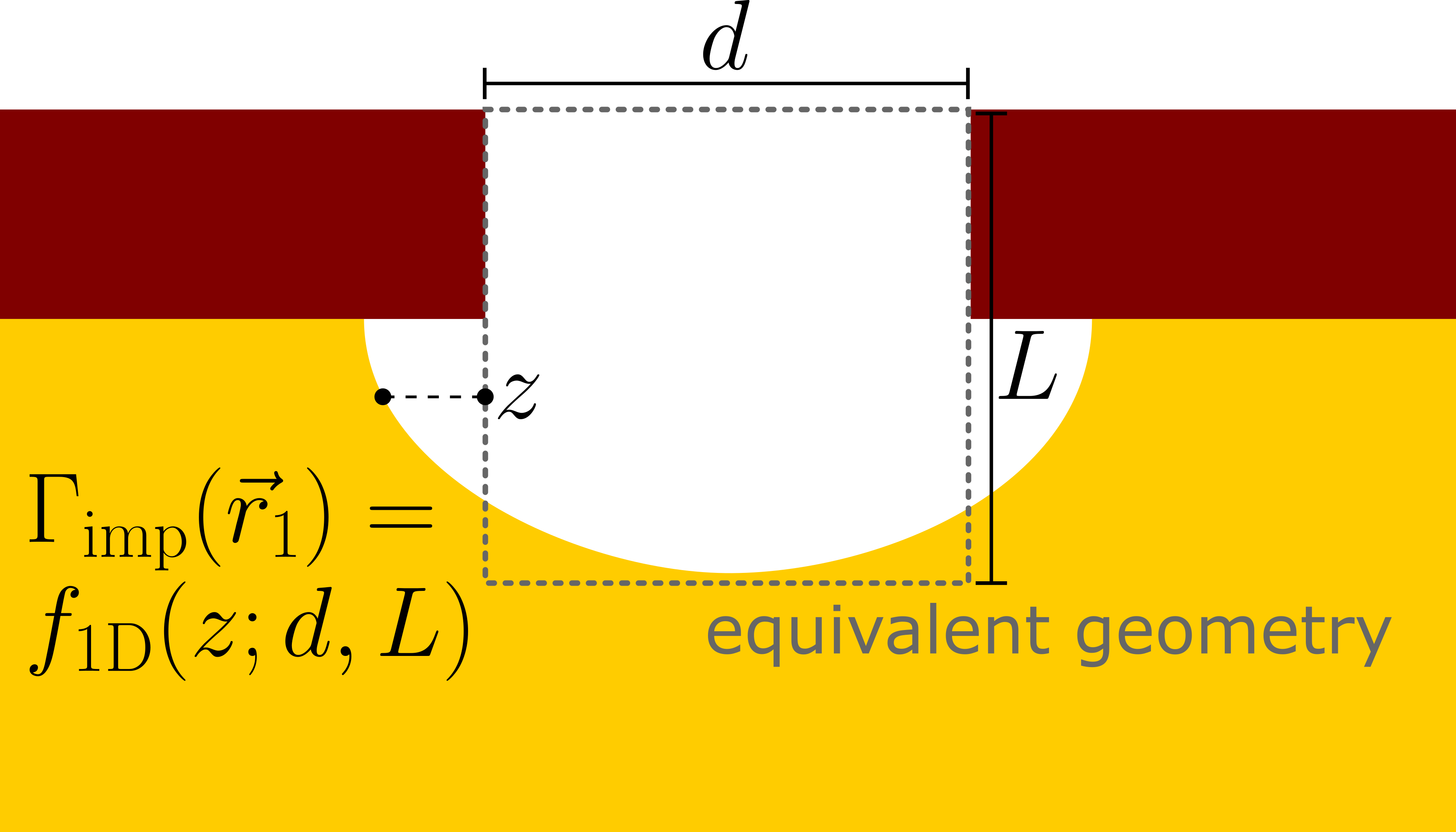
The flux calculation approaches hitherto discussed can be computationally challenging for arbitrary three-dimensional (3D) geometries, even with relatively simple surface kinetics such as the constant $\beta$ approximation. However, in many situations encountered in semiconductor fabrication, symmetry considerations and approximations can be made to reduce the dimensionality of the problem from 3D to 1D, particularly for structures involving high aspect ratios (ARs) and a preferential transport direction. The AR is defined as the ratio between two critical dimensions (CDs): Depth $L$ to width $d$ (c.f. Fig. 2.7)

$$\begin{array}{}\text{(2.19)}& \text{AR}=\frac{L}{d}.\end{array}$$

For example, trenches and vias necessary for innovative back end of line (BEOL) processing [104] as well as modern 3D NAND memories [105] require increasingly higher ARs. Although such structures can have intricate shapes, it is often more useful to focus on phenomena due to the high AR itself. Thus, the complex structure under investigation is replaced by a simpler equivalent geometry with well-defined CDs, as illustrated in Fig. 2.7. Therefore, 1D models with faster performance and additional physical insight can be constructed.

The key approximation behind all 1D models is the assumption that all reactants have an isotropic source distribution and also reflect isotropically (e.g., Eq. (2.12)). This greatly simplifies Eq. (2.14) which takes the form of an integral equation over the whole structure area $A^{\prime }$ [106]

$$\begin{array}{}\text{(2.20)}& {\mathrm{\Gamma }}_{\mathrm{imp}}(\overrightarrow{r})={\mathrm{\Gamma }}_{\mathrm{vis}}(\overrightarrow{r})+{\int }_{A^{\prime }}(1-\beta ({\overrightarrow{r}}^{\prime })){\mathrm{\Gamma }}_{\mathrm{imp}}({\overrightarrow{r}}^{\prime })\frac{⟨(\overrightarrow{r}-{\overrightarrow{r}}^{\prime }),{\overrightarrow{n}}^{\prime }⟩⟨({\overrightarrow{r}}^{\prime }-\overrightarrow{r}),\overrightarrow{n}⟩}{\pi ||\overrightarrow{r}-{\overrightarrow{r}}^{\prime }|{|}^4}d{A}^{\prime }\end{array}$$ and is named the radiosity equation, highlighting that the problem is entirely analogous to diffuse radiative heat transfer [98]. This equation can be directly solved using finite elements for arbitrary geometries at great computational cost [97]. However, the problem can be simplified by identifying the view factor in Eq. (2.20), which is the fraction of energy $d{F}_{d{A}^{\prime }-dA}$ leaving one differential surface $d{A}^{\prime }$ and arriving in $dA$ separated by a distance $t$, as follows [98]

$$\begin{array}{}\text{(2.21)}& d{F}_{d{A}^{\prime }-dA}=\frac{⟨(\overrightarrow{r}-{\overrightarrow{r}}^{\prime }),{\overrightarrow{n}}^{\prime }⟩⟨({\overrightarrow{r}}^{\prime }-\overrightarrow{r}),\overrightarrow{n}⟩}{\pi ||\overrightarrow{r}-{\overrightarrow{r}}^{\prime }|{|}^4}d{A}^{\prime }=\frac{\cos \theta \cos {\theta }^{\prime }}{\pi t^2}d{A}^{\prime }.\end{array}$$

In Eq. (2.21), $\theta$ are the angles between each surface normal and the line connecting the surface elements. Thus, pre-calculated tables of view factors [107] can be used to map common high AR structures to 1D line equations over the preferential transport direction $z$. This enabled Manstetten et al. to construct an 1D framework which calculates the flux for several convex high AR structures under the constant $\beta$ approximation [108]. Kokkoris et al. created similar equations for long cylindrical holes and trenches, while also enabling locally-varying $\beta (\overrightarrow{r})$ though a self-consistent calculation [106].

These 1D radiosity approaches are valuable due to their computational efficiency. However, they still require a costly matrix inversion step for the calculation of the local fluxes which might be performed several times in the self-consistent calculation for varying $\beta (\overrightarrow{r})$. Additionally, these approaches do not enable an intuitive understanding of the effects of the reactive transport parameters without performing the simulations. This motivates another type of 1D model where, instead of directly calculating the integral equation, the reactive transport process is approximated with an 1D diffusion equation [30]. This diffusive transport approach is, however, not only based on conventional molecule-molecule (Fickian) diffusion. Instead, the main drivers of the diffusive process are the molecule-geometry interactions in a process called Knudsen diffusion, which is explored in detail in Chapter 3, including an approach to model the transitional flow regime.