The drift-diffusion equations for spin in metallic FM systems were first derived by T. Valet and A. Fert using a spin generalized Boltzmann equation [59], which described systems with collinear magnetic regions. Later, a
drift-diffusion formalism generalized for arbitrary magnetization directions was presented by S. Zhang, P. Levy, and A. Fert [57]. In this section, the main results of the Zhang-Levy-Fert model are summarized, together with
extensions to the model which form the basis for the spin torque computation framework used in this work.
The response of the current density to an applied electric field along \(x\) in a FM layer is considered. In the linear response regime, the currents along \(x\) can be expressed as follows [57]
The function \(E_x(x) = -\partial _x V(x)\) is the local electric field, given by the partial derivative along \(x\) of the local electrical potential \(V(x)\). The matrices \(\hat {C}\) and \(\hat {D}\) are spin generalized
conductivity and diffusion coefficient matrices, respectively, and \(\hat {n}(x)\) is the charge-spin accumulation at a given position. For metals, the diffusion coefficient and conductivity are related to each other via the Einstein
relation: \(\hat {C} = e^2\hat {N}(\epsilon _F )\hat {D}\), where \(\hat {N}(\epsilon _F )\) is the DOS at the Fermi level. The diffusion coefficient, conductivity, and accumulation can be expanded in Pauli matrices:
\(\seteqnumber{1}{4.7}{0}\)
\begin{align}
\hat {C} = C_0 \hat {1} + \bm {\hat {\sigma }} \cdot \bm {C}, \\ \hat {D} = D_0 \hat {1} + \bm {\hat {\sigma }} \cdot \bm {D}, \\ \hat {n} = n_0 \hat {1} + \bm {\hat {\sigma }} \cdot \bm {s},
\end{align}
where \(2n_0\) is the charge accumulation and \(\bm {s}\) is the non-equilibrium spin accumulation, which describes the net spin polarization and is only present when an electric field is applied. The magnetic moment of the
non-equilibrium spin accumulation is obtained by multiplying the spin accumulation by \(-\mu _B/e\). \(C_0\) and \(D_0\) are related to the electrical conductivity and electron diffusion coefficient by \(\sigma = 2C_0\) and
\(D_e = 2D_0 \), respectively. The conductivity and diffusion coefficient, are related to the majority/minority conductivity \(\sigma ^{\uparrow /\downarrow }\) and diffusion coefficient \(D_e^{\uparrow /\downarrow }\), by
\(\sigma = (\sigma ^{\uparrow }+\sigma ^{\downarrow })/2\) and \(D_e = (D_e^{\uparrow }+D_e^{\downarrow })/2\), respectively. The spin-dependent parts of the conductivity and diffusion coefficient are given by
\(\bm {\hat {C}} = -\beta _\sigma C_0\bm {m}\) and \(\bm {\hat {D}}= -\beta _D D_0\bm {m}\), where \(\beta _\sigma = (\sigma ^\uparrow -\sigma ^\downarrow )/(\sigma ^\uparrow +\sigma ^\downarrow
)\) and \(\beta _D = (D_e^\uparrow -D_e^\downarrow )/(D_e^\uparrow +D_e^\downarrow )\) are conductivity and diffusion polarizations, respectively. The conductivity and diffusion polarizations are only equal when the
DOS are the same for majority and minority electrons, otherwise \(\beta _\sigma \neq \beta _D\).
Expanding the current density along x in Pauli matrices, yields
where, the spin polarization current density \((\bm {j_{sx}})_i = j_{ix}\) describes the flow of spin angular momentum component \(i\) along \(x\). The charge and spin current densities in real space are then obtained by
taking the trace over the spin space, which gives
\(\seteqnumber{1}{4.9}{0}\)
\begin{align}
j_{cx}(x) = \text {Tr}[\hat {j}_x] = \sigma E(x) - \beta _D D_e \bm {m}\cdot \partial _x\bm {s}(x), \\ \bm {j_{sx}}(x) = \text {Tr}[\bm {\hat {\sigma }}\hat {j}_{x}]= \beta _\sigma \bm
{m}(\sigma E(x)) -D_e\partial _x\bm {s}(x).
\end{align}
The \(\partial _x n_0\) terms were omitted as the distribution of charges in a metal (except within a screening length from an interface or free surface) can be considered uniform [60]. Repeating these steps for an electric field
along the \(y\) and \(z\) directions, and omitting the position dependence for brevity, the equations can be extended to three dimensions:
\(\seteqnumber{1}{4.10}{0}\)
\begin{align}
\label {eq:charge_current_wo_SHE} \bm {j_c} & = \sigma \bm {E} - \beta _D D_e (\nabla \bm {s})^T\bm {m}, \\ \tilde {j}_s & = \beta _\sigma \bm {m} \otimes (\sigma \bm {E}) -D_e(\nabla
\bm {s}).
\end{align}
Here the tensor spin polarization current \((\tilde {j}_{s})_{ij}\) is introduced, describing the flow of polarization component \(i\) along direction \(j\). The tilde \(\tilde {\,}\) denotes a \(3\times 3 \) matrix,
\(\,^T\) denotes the matrix transpose, \(\otimes \) is the outer product such that \((\bm {m} \otimes \bm {E})_{ij} = m_i E_j \), and \((\nabla \bm {s})_{ij} = \partial _j s_i \) is the vector gradient of the spin
accumulation. The electric field in three dimensions is given by \(E = -\nabla V\). For a NM layer Eq. 4.10 holds for \(\bm {m} = 0\).
As the ultimate goal is to couple the drift-diffusion equations with magnetization dynamics, it is convenient to express the spin polarization current and the spin accumulation in terms of the magnetic moment carried by the spin.
This is achieved by introducing the spin magnetic moment accumulation \(\bm {S} = -(\mu _B/e)\bm {s}\), and the spin magnetic moment current density \(\tilde {J_{s}} = -(\mu _B/e)\tilde {j_{s}}\), which are in
units of A/m and A/s, respectively. The charge and spin current densities can then be expressed as
\(\seteqnumber{1}{4.11}{0}\)
\begin{align}
j_{c} = \sigma E + \frac {e}{\mu _B}\beta _D D_e(\nabla \bm {S})^T\bm {m}, \\ \tilde {J_{s}} =-\frac {\mu _B}{e}\beta _\sigma \bm {m} \otimes (\sigma \bm {E}) -D_e(\nabla \bm {S}).
\end{align}
For brevity, \(\bm {S}\) and \(\tilde {J_{s}} \) will be referred to as just the spin accumulation and spin current, respectively.
4.2.1 Continuity Equations
In NM and FM layers, due to bulk spin-flip processes caused by bulk SOC, magnetic impurities, and disorder, the non-equilibrium spin accumulation loses its polarization over time scales characterized by the spin-flip time \(\tau
_{sf}\). Moreover, in the bulk of FM layers, the electron’s spin interacts with the local magnetization through the s-d exchange interaction described by the Hamiltonian term
where \(J\) is the s-d exchange coupling constant. When the spin accumulation and magnetization are not parallel, spin angular momentum is transferred from the spin accumulation to the magnetization through this interaction.
Taking these losses into account, the continuity equation for the spin accumulation can be expressed as
where the first term on the right-hand side describes the decay of spin accumulation due to spin-flip scattering, while the second term describes the precessional motion of the spin accumulation around the magnetization induced by
the exchange interaction.
Typically, the dynamics of the spin accumulation occur over timescales in the order of femtoseconds, while magnetization dynamics occur over timescales in the order of picoseconds [57]. Therefore, the spin accumulation can be
considered to be in quasi-static equilibrium with the magnetization. This allows the time derivative of the spin accumulation to be neglected; thus, the continuity equation can be written as
where the length parameters \(\lambda _{sf} = \sqrt {D_e\tau _{sf} } \), \(\lambda _{sf} = \sqrt {D_e\hbar /J}\), were introduced, which are referred to as the spin-flip and exchange length, respectively. The validity
of this assumption was verified numerically by coupling Eq. (4.14) with the LLG equation in [61].
The continuity equation for the charge current density is obtained by taking the divergence of Ampere’s law and using Gauss’s law to express the divergence of the displacement field in terms of the charge density:
\(\seteqnumber{0}{4.}{14}\)
\begin{align}
\nabla \cdot \left (\partial _t \bm {D} + \bm {j_c}\right ) = \nabla \cdot \left (\nabla \times \bm {H} \right ) & = 0, \\ \partial _t \rho _c + \nabla \cdot \bm {j_c} & = 0.
\end{align}
For a steady current, the charge density is constant, thus the time derivative can be omitted, yielding
Another mechanism contributing to the decay of transverse spin components is spin dephasing. Spin dephasing arises when spins precess by varying amounts after traveling a certain distance, leading to the cancellation of their
transverse components. This phenomenon can occur due to variations in electron velocities across the Fermi surface or due to spins precessing at the same rate but arriving at different times as a result of spin-dependent scattering.
The behavior of the spin accumulation, incorporating both precessional and dephasing effects, was treated using the Continuous Random Matrix Theory (CRMT) in [62], where the equivalence between the CRMT and the charge
and spin drift-diffusion approach was shown. To account for the spin dephasing, the continuity equation for the spin accumulation is expanded by including an additional term orthogonal to the spin exchange term:
Here, the length parameter \(\lambda _\phi = (l_\perp /l_L) \lambda _J \), referred to as the dephasing length, is introduced. The parameters \(l_\perp \) and \(l_J\) relating the dephasing length to the exchange length
are the spin coherence length and spin precession lengths, respectively, which can be extracted from ab initio data [63].
4.2.3 Spin Torque
Both the exchange and dephasing terms describe a process that transfers angular momentum from the spin accumulation to the magnetization. This transfer of angular momentum can be interpreted as a torque acting on the
magnetization. The torque expression can be derived from Eq. (4.18) by applying the principle of angular momentum conservation [63].
Slonczewski’s original work [29] proposed that the divergence of the spin current, representing the angular momentum lost by the conduction electrons, must correspond to the angular momentum gained by the magnetization. This
holds true in the absence of additional spin relaxation mechanisms [64]. However, the spin-flip relaxation term describes processes that do not contribute to the torque on the magnetization. The main contribution is due to the
SOC, which transfers part of the electron’s angular momentum to the crystal lattice [63, 65]. Spin-flip scattering of magnetic impurities and disorder can also contribute to the spin-flip relaxation [65]. Thus, the resulting
position-dependent torque can be expressed in units of A/(ms) as
The total torque acting on the magnetization of a FM layer is obtained by integrating the position-dependent torque over the volume of the layer.
4.2.4 The Direct and Inverse SHE
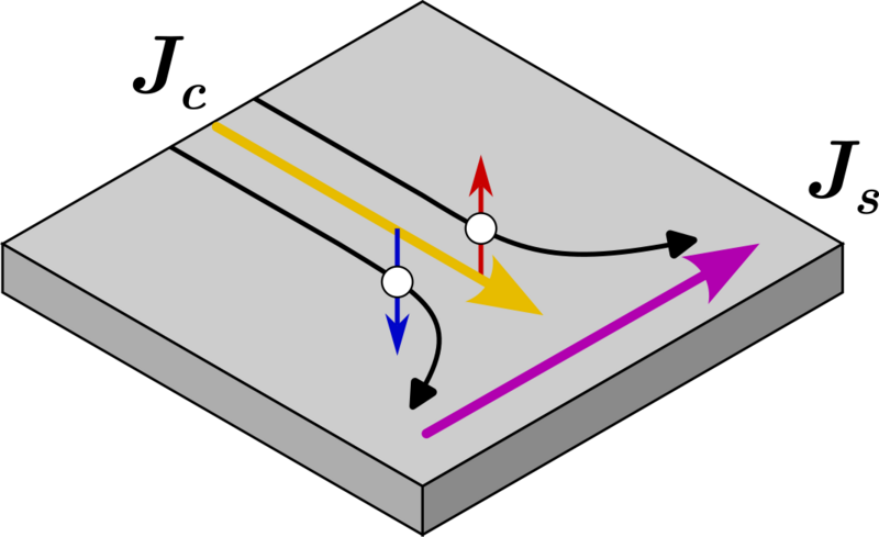
(a) The spin Hall effect.
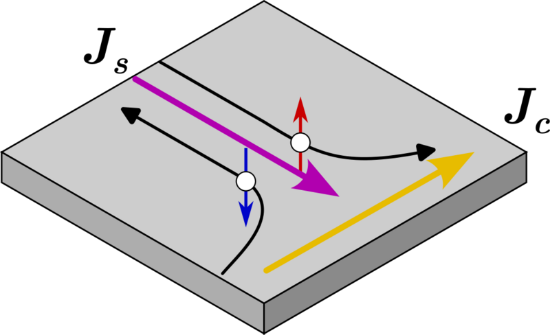
(b) The inverse spin Hall effect.
Figure 4.1: Illustration of the SHE (a) and ISHE (b). The SOC deflects electrons in opposite directions depending on their spin, generating a spin current from an applied charge current (a) or a charge current from an injected
spin current (b).
In the bulk of NM HMs, when an electric field is applied, the SOC in the band structure and at defects drives the SHE. The resulting pure spin current is transverse to the charge current, with a polarization direction perpendicular
to both. Reciprocally, a pure spin current can generate a charge current through the ISHE. Both effects are depicted in Fig. 4.1. The SHE and ISHE can be described by extending
the definitions of the charge and spin currents [66, 54]:
\(\seteqnumber{1}{4.20}{0}\)
\begin{align}
(j_c)_i & = (j_c^0)_i + \frac {e}{\mu _B}\alpha _\mathrm {SH}\varepsilon _{ijk}(\tilde {J}^0_s)_{jk}, \\ (\tilde {J}_s)_{ij} & = (\tilde {J}^0_s)_{ij} - \frac {\mu _B}{e}\alpha
_\mathrm {SH}\varepsilon _{ijk}(\tilde {j}^0_c)_{k}.
\end{align}
The superscript \(0\) denotes the currents without the SHE, \(\varepsilon _{ijk}\) is the Levi-Civita symbol capturing the orthogonality of the spin Hall currents, and \(\alpha _\mathrm {SH}\) is a dimensionless coupling
parameter capturing the strength of the bulk spin-orbit interaction referred to as the spin Hall angle. The spin Hall angle can be calculated using ab initio methods, or be extracted from experiments, and is typically on the
order of tens of percent for HMs such as Pt, Ta, and W [67]. The spin Hall angle is often used as a measure of the efficiency of the charge-to-spin conversion, and can be defined as the ratio of the transverse spin current to the
longitudinal charge current. The spin Hall angle can be expressed in terms of the spin Hall conductivity \(\sigma _\mathrm {SH}\) as \(\alpha _\mathrm {SH} = \sigma _\mathrm {SH}/\sigma \).
\begin{align}
\label {eq:charge_current_with_SHE} \bm {j_{c}} & = \sigma \bm {E} + \frac {e}{\mu _B}\beta _D D_e (\nabla \bm {S})^T\bm {m} + \frac {e}{\mu _B}\alpha _\mathrm {SH}D_e(\nabla \times \bm
{S}) , \\ \label {eq:spin_current_with_SHE} \tilde {J}_s & = -D_e\nabla \bm {S} - \frac {\mu _B}{e}\beta _{\sigma }\bm {m} \otimes (\sigma \bm {E}) - \frac {\mu _B}{e}\alpha _\mathrm
{SH}\varepsilon (\sigma \bm {E}),
\end{align}
where \((\varepsilon \bm {E})_{ij} = \varepsilon _{ijk}E_k \). The last term in the expression for the electrical current describes the ISHE, obtained from the curl of the spin accumulation, while the last term in the
expression for the spin current describes the direct SHE, generated by the electric field.