In 1857, William Thomson (Lord Kelvin) discovered that when iron and nickel were subjected to an external magnetic field, the electrical resistance would increase or decrease depending on the orientation of the field relative to the
direction of the current through the material [15]. In ferromagnets, this phenomenon is known as the anisotropic magnetoresistance (AMR) and is attributed to the combined action of the magnetization and the SOC on the
scattering of conduction electrons. Several other forms of magnetoresistance have been discovered since then, most notably the giant magnetoresistance (GMR) and tunneling magnetoresistance (TMR), which are often considered to
be the origin of the field of spintronics.
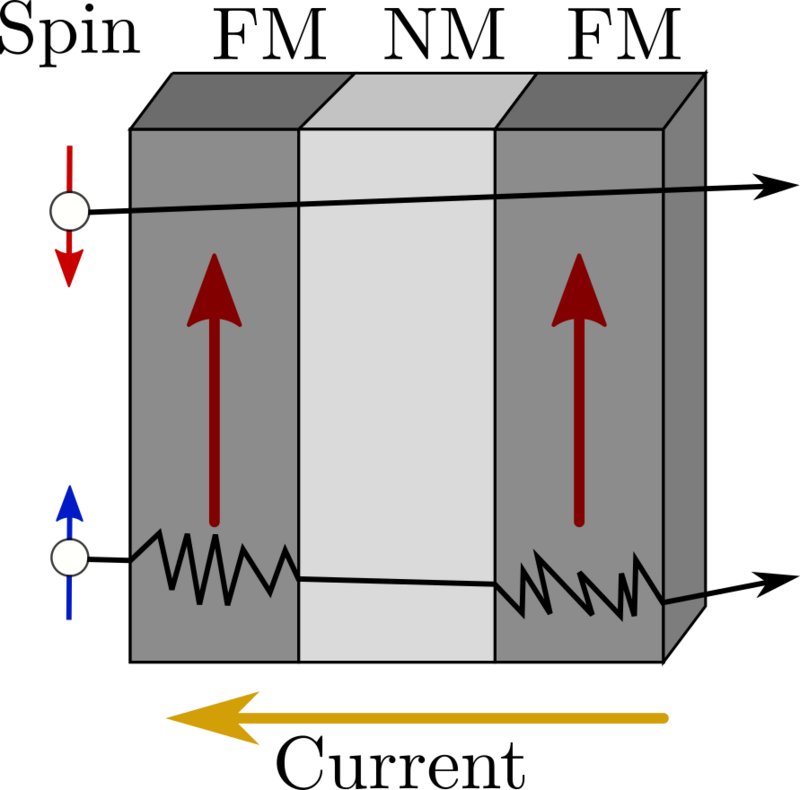
(a) Parallel
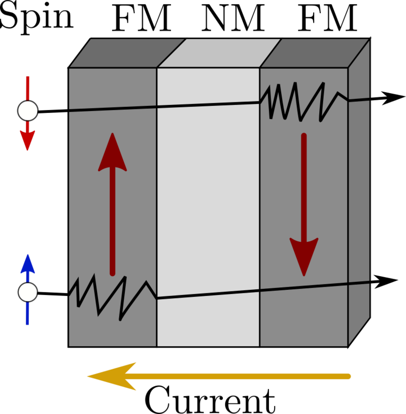
(b) Antiparallel
Figure 2.1: Visual depiction of the GMR effect in a spin valve. The magnetic state of the two FM layers is indicated by the red arrows. In the parallel configuration (a), the resistance is low, while in the antiparallel configuration
(b), the resistance is high due to spin-dependent scattering.
The GMR was discovered independently by two research groups led by Albert Fert in France and Peter Grünberg in Germany in 1988 [17, 18]. The practical significance of the discovery resulted in both being awarded the
2007 Nobel Prize in Physics. The GMR effect occurs in metallic multilayers composed of alternating FM and NM thin films. In these systems, the electrical resistance depends strongly on the relative orientation of the magnetizations
in the FM layers. When the magnetizations are aligned parallel, the resistance is low, while when they are aligned antiparallel, the resistance is high. The effect originates from spin-dependent electron scattering in the FM layers.
The simplest structure exhibiting GMR is a spin valve, consisting of two FM layers separated by an NM spacer layer (SL). Figure 2.1 shows a schematic of the spin flow in a
spin valve. When the two FM layers have a parallel configuration, the majority conduction electrons scatter less than the minority electrons, resulting in a lower overall resistance. In the antiparallel configuration, both spin channels
experience significant scattering, resulting in higher resistance. As the resistance ratio between the two configurations is typically in the order of a few tens of percent, much higher than the AMR in pure magnetic metals (typically
\(\approx 1\%\)), the effect is termed "giant" magnetoresistance. As a higher resistance ratio enabled better signal detection, GMR quickly found applications in magnetic field sensors and hard disk read heads, revolutionizing
data storage technology [19]. However, the low magnetoresistance ratio limited the potential memory applications.
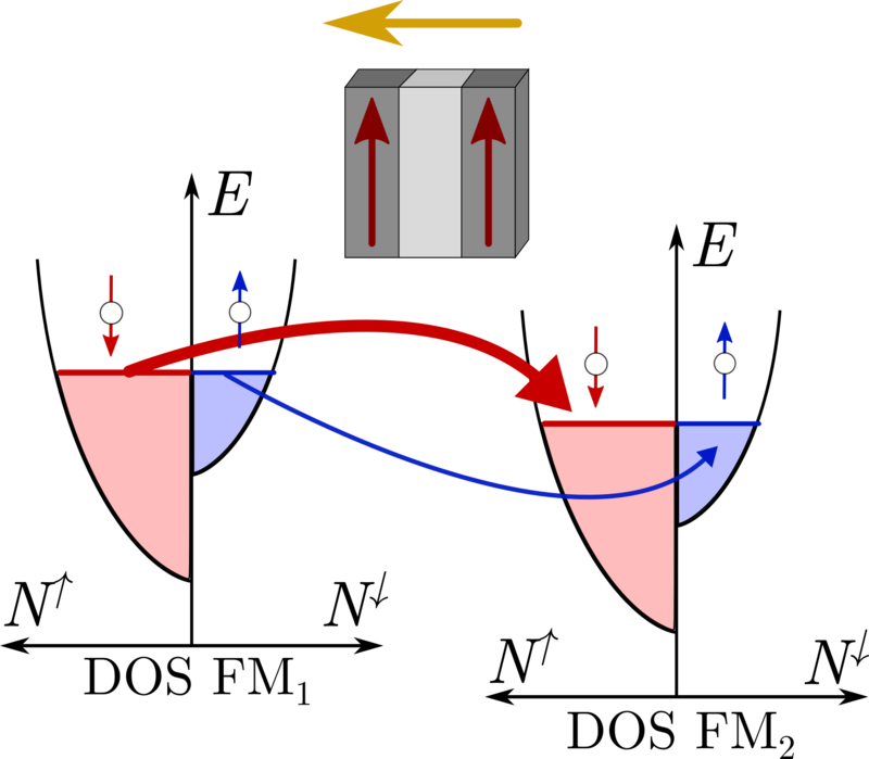
(a) Parallel
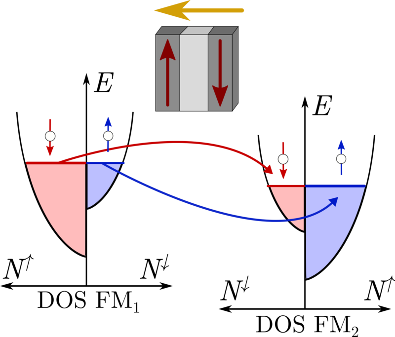
(b) Antiparallel
Figure 2.2: Schematic of the TMR effect in a MTJ. The magnetic state of the two FM layers and the current direction are indicated by the red and yellow arrows, respectively. In the parallel configuration (a), the majority
and minority spin bands of the two FM layers match, which facilitates tunneling and leads to a low resistance state, while in the antiparallel configuration (b), the bands are misaligned, resulting in a high resistance.
Another type of magnetoresistance, which was discovered over a decade earlier in 1975 by Michel Jullière, is the TMR [20]. The TMR effect is observed in magnetic tunnel junctions (MTJs), which consist of two FM layers separated
by a thin insulating layer referred to as the tunnel barrier (TB). The TMR is caused by spin-dependent tunneling and depends on the difference in the Fermi level density of states (DOS) between the spin-up and spin-down
electrons. The tunneling probability depends on the relative orientation of the magnetizations in the FM layers, resulting in a change in resistance similar to that of GMR.
Figure 2.2 shows a schematic of the TMR effect. When the thickness of the TB is sufficiently thin (typically in the order of a few nanometers), electrons can tunnel quantum
mechanically through the barrier, depending on the available conduction states in the adjacent FM layer. Since the tunneling preserves the electron’s spin, the electrons can only tunnel to a band of the same spin orientation. In the
parallel state, the majority and minority spin bands of the two FM layers match, allowing electrons to tunnel through the barrier with a higher probability, resulting in a lower resistance. In the antiparallel configuration, the spin
bands do not match, reducing the tunneling probability and leading to a higher resistance.
Initially, the effect received little attention due to its low resistance ratios (a few percent at low temperatures) and the difficulty in fabricating high-quality tunnel junctions. However, in 1995, the discovery of large TMR effects in
MTJs with amorphous Al\(_2\)O\(_3\) barriers at room temperature by Miyazaki et al. and Moodera et al. sparked renewed interest in the phenomenon [21, 22]. Theoretical predictions suggested that using
crystalline MgO barriers could lead to even higher TMR ratios due to coherent tunneling processes [23, 24]. This was experimentally confirmed in the middle of the 2000s when TMR ratios exceeding \(200\%\) at room temperature
in Fe/MgO/Fe and CoFeB/MgO/CoFeB MTJs were reported [25, 26, 27]. The high TMR ratios achieved with MgO barriers made MTJs highly compatible with standard CMOS technology, and thus attractive for applications such
as MRAM.
Together, the GMR and TMR enabled the possibility of storing logical states in the relative magnetization orientation of FM layers, which could be easily distinguished electrically through simple resistance measurements. Because
the magnetization states remain stable without a continuous power supply, such magnetic data storage is inherently non-volatile, making it especially attractive for memory applications. A common example is the antiparallel and
parallel states of a spin-valve or MTJ, which represent the binary states "0" and "1", respectively. In this case, the magnetization of one layer is fixed, while the magnetization of the other layer can be switched between parallel and
antiparallel states, representing the binary states "0" and "1". These two FM layers are therefore referred to as the reference layer (RL) and free layer (FL), respectively. The RL magnetization is typically pinned by exchange bias
with an adjacent synthetic AFM layer. To retain the bit information at a wide range of temperatures while allowing switching, an uniaxial magnetic anisotropy is introduced to the FL, either through the shape of the layer or
through interfacial effects, such that the two states are energetically favorable and separated by an energy barrier \(E_B\). The thermal stability of the stored information is characterized by the thermal stability factor \(\Delta =
E_B/(k_B T)\), where \(k_B\) is the Boltzmann constant and \(T\) is the temperature. A 10-year data retention on a bit level, typically requires a minimum thermal stability factor of \(40\) for a MTJ [28], which increases with
the memory capacity.