Modeling Spin-Orbit Torques
in Advanced Magnetoresistive Devices

5.3 Effective Interface Field Model

The perturbation theory description of interfacial SOC introduces a modification of the unperturbed scattering matrices, which allows for the SOC to be treated for various types of interfaces with magnetism, such as topological insulator/FM or NM/FM insulator interfaces, in addition to the typical metallic NM/FM bilayers [77]. However, it is only valid when the spin-orbit interaction is weak relative to the bulk s-d exchange interaction, such that the projection of the spin onto the magnetization direction is a good approximation. To treat the opposite case where the SOC dominates, a different approach is required. In this section, the case of a NM/FM interface where an effective magnetic field located at the interface dominates over the bulk exchange interaction is considered. This effective field can comprise both an interfacial exchange interaction between the electron’s spin and the magnetization at the interface, as well as a momentum-dependent spin-orbit field. In this case, the spins can be projected along the direction of the effective field at the interface, allowing for the strong SOC regime to be treated non-perturbatively. The following three subsections were adapted from Ref. [79].

5.3.1 Interface Model

An interface at \(z=0\) with an effective magnetic field \(\bm {B}\), separates a metallic FM layer (\(z > 0\)) from a metallic NM layer (\(z < 0\)). Assuming the exchange splitting in the bulk of the FM layer is weak relative to the exchange splitting caused by the effective interface field, the NM and FM bulk can be treated as a spin-independent free electron gas. For simplicity, the same Fermi wave vector and effective mass are assumed on either side of the interface. The interface is modeled as a zero-thickness region described by a delta function potential barrier at \(z=0\), which contains a spin-independent potential with energy \(V_0 = \hbar ^2k_F u_0/m_e\), and a spin-dependent exchange interaction between the electron’s spin and the effective magnetic field at the interface with energy \(J_\mathrm {ex} = \hbar ^2k_F u_{ex}/m_e\), where \(u_0\) and \(u_\mathrm {ex}\) are the dimensionless magnitudes of each potential. The Hamiltonian describing this system is given by

\begin{equation} \hat {H}=-\frac {\hbar ^2}{2 m_e} \nabla ^2+ \delta (z)\left (V_0\hat {1} + J_\mathrm {ex}\bm {\hat {\sigma }}\cdot \bm {b} \right ). \end{equation}

The vector \(\bm {b}= \bm {B}/B\) is the normalized direction of the effective magnetic field at the interface. Electrons incident on the interface experience different potential barriers \(U^{\uparrow /\downarrow } = V_0 \mp J_\mathrm {ex}\) at the interface, depending on their spin projection along the effective interface field. Thus, the electrons can be split into majority and minority species, depending on their spin being antiparallel (\(\uparrow \)) or parallel (\(\downarrow \)) to \(\bm {b}\), respectively. It should be noted that in this model, there is no explicit distinction between the two sides of the interface in the Hamiltonian. Instead, the difference between the NM and FM bulk will be described by their respective non-equilibrium distribution functions.

Using plane-wave solutions of the time-independent Schrödinger equation and assuming specular scattering at the interface, the following reflection and transmission amplitudes for majority/minority electrons are obtained [80]:

\begin{equation} \label {eq:scattering_matricies_amin} r_{\bm {k}}^{\uparrow / \downarrow } =\frac {u^{\uparrow /\downarrow }}{ i (k_z/k_F)-u^{\uparrow /\downarrow }}, \quad \text {and}\quad t_{\bm {k}}^{\uparrow / \downarrow } =\frac { i (k_z/k_F)}{ i (k_z/k_F)-u^{\uparrow /\downarrow }}, \end{equation}

respectively, where \(u^{\uparrow /\downarrow } = u_0 \mp u_{ex}\) is the dimensionless majority/minority potential barrier. The corresponding scattering matrices can be expressed in spin space in terms of spin projection matrices:

\begin{equation} \label {eq:expanded_scattering_matricies} \hat {r}_{\bm {k}} = \sum _s \hat {p}^s r_{\bm {k}}^s,\quad \text {and}\quad \hat {t}_{\bm {k}} = \sum _s \hat {p}^s t_{\bm {k}}^s, \end{equation}

for \(s\in \{\uparrow ,\downarrow \}\), where \(\hat {p}^{\uparrow /\downarrow } = (\hat {1} \mp \bm {\hat {\sigma }}\cdot \bm {b})/2\) is the spin projection matrix along the effective field for majority/minority carriers.

The analysis thus far remains unchanged if the interfacial effective magnetic field is allowed to depend on momentum, i.e., \(\bm {b}\rightarrow \bm {b}_{\bm {k}}\). Consequently, the scattering amplitudes and projections also become momentum dependent: \(u^{\uparrow /\downarrow }\rightarrow u^{\uparrow /\downarrow }_{\bm {k}}\), \(\hat {p}^{\uparrow /\downarrow }\rightarrow \hat {p}^{\uparrow /\downarrow }_{\bm {k}}\). The effective field is then assumed to consist of two parts: a momentum-independent interfacial exchange coupling between the electron spin and the magnetization at the interface, with associated energy \(J_m =\hbar ^2k_F u_{m}/m_e\); and a momentum-dependent spin-orbit contribution along \(\bm {b^{\mathrm {SO}}_{\bm {k}}}\) with energy \(J_\mathrm {SO}=\hbar ^2k_F u_\mathrm {SO}/m_e\), where the parameters \(u_m\) and \(u_\mathrm {SO}\) are the respective dimensionless interaction strengths. Consequently, the orientation of the total effective field is given by

\begin{equation} \bm {b_k} = (J_m\bm {m} + J_\mathrm {SO}\bm {b^{\mathrm {SO}}_{\bm {k}}})/J_\mathrm {ex}, \end{equation}

with \(J_\mathrm {ex} = \| J_m\bm {m} + J_\mathrm {SO}\bm {b^{\mathrm {SO}}_{\bm {k}}}\|\). In this framework, various spin-orbit fields can be incorporated, such as Rashba or Dresselhaus types or linear combinations thereof.

5.3.2 Charge and Spin Currents

Since the scattering matrices are the same for both sides of the interface, i.e. \(\hat {t}_{\bm {k}} = \hat {t}^\prime _{\bm {k}}\) and \(\hat {r}_{\bm {k}} = \hat {r}^\prime _{\bm {k}}\), the out-of-plane current densities at either side of the interface cas be written as

\begin{equation} \label {eq:landauer_butikker_2} \hat {j}_z(0^{\mathbin {\textpm }})= {\mathbin {\textpm }}\frac {e}{h A} \sum _{\bm {k_\|}\in \mathrm {FS}} \left [\hat {g}_{\bm {k}}^{\mathrm {F/N}} -\hat {r}_{\bm {k}} \hat {g}_{\bm {k}}^{\mathrm {F/N}} \hat {r}_{\bm {k}}^{\dagger }-\hat {t}_{\bm {k}} \hat {g}_{\bm {k}}^{\mathrm {N/F}} \hat {t}_{\bm {k}}^{\dagger } \right ]. \end{equation}

Expanding the scattering matrices in terms of the spin projection matrices, one obtains

\begin{equation} \label {eq:landauer_butikker_3} \hat {j}_z(0^{\mathbin {\textpm }}) = \frac {1}{eA}\sum _{\bm {k_\|}\in \mathrm {FS}} \left [\mathcal {G}^{\uparrow \uparrow }_{\bm {k}}\hat {p}_{\bm {k}}^\uparrow \Delta \hat {g}_{\bm {k}}\hat {p}_{\bm {k}}^\uparrow + \mathcal {G}^{\downarrow \downarrow }_{\bm {k}}\hat {p}_{\bm {k}}^\downarrow \Delta \hat {g}_{\bm {k}}\hat {p}_{\bm {k}}^\downarrow {\mathbin {\textpm }} \mathcal {G}^{\uparrow \downarrow }_{\bm {k}}\hat {p}_{\bm {k}}^\uparrow \hat {g}_{\bm {k}}^{\mathrm {F/N}}\hat {p}_{\bm {k}}^\downarrow {\mathbin {\textpm }} (\mathcal {G}^{\uparrow \downarrow }_{\bm {k}})^*\hat {p}_{\bm {k}}^\downarrow \hat {g}_{\bm {k}}^{\mathrm {F/N}}\hat {p}_{\bm {k}}^\uparrow \mp \mathcal {T}^{\uparrow \downarrow }_{\bm {k}}\hat {p}_{\bm {k}}^\uparrow \hat {g}_{\bm {k}}^{\mathrm {N/F}}\hat {p}_{\bm {k}}^\downarrow \mp (\mathcal {T}^{\uparrow \downarrow }_{\bm {k}})^*\hat {p}_{\bm {k}}^\downarrow \hat {g}_{\bm {k}}^{\mathrm {N/F}}\hat {p}_{\bm {k}}^\uparrow \right ], \end{equation}

where \(\Delta \hat {g}_{\bm {k}} = \hat {g}^F_{\bm {k}}-\hat {g}^N_{\bm {k}} \). Here, the momentum-resolved spin-dependent conductances for reflection and transmission \(\mathcal {G}^{ss^\prime }_{\bm {k}} = e^2/h[1 - r^{s}_{\bm {k}}(r_{\bm {k}}^{s^\prime })^*]\) and \(\mathcal {T}^{ss^\prime }_{\bm {k}} = e^2/h[t^{s}_{\bm {k}}(t_{\bm {k}}^{s^\prime })^*]\) are introduced, for \(s, s^\prime \in \{\uparrow ,\downarrow \}\).

Inserting the expression for the non-equilibrium distribution function (5.4) for an in-plane electric field \(E_x\) along \(\bm {x}\) into Eq. (5.33) and performing the trace over the spin components, allows for the momentum dependence to be factorized. Thus, one can express the charge and spin currents in terms of momentum-averaged conductance and conductivity tensors:

\begin{equation} j_{zc}(0^{\mathbin {\textpm }}) = G_{+}\Delta V_{c} + \bm {G_{-}}\cdot \Delta \bm {V_{s}} + \Delta \sigma _+ E_x + \beta _{\tau }(\bm {\sigma _{-}^F}\cdot \bm {m})E_x, \end{equation}

\begin{equation} \label {eq:spin_currents_p} \bm {J_{zs}}(0^+) =\frac {\mu _B}{e}\left [ \tilde {G}_{+}\Delta \bm {V_{s}} +\bm {G_{-}}\Delta V_{c} - \tilde {G}_{\uparrow \downarrow }\bm { V_{s}^{\mathrm {F}}} + \tilde {\Gamma }_{\uparrow \downarrow }\bm { V_{s}^{\mathrm {N}}} +\Delta \bm {\sigma _{-}}E_x +\beta _{\tau }(\tilde {\sigma }^F_{+}-\tilde {\sigma }^F_{\uparrow \downarrow })\bm {m}E_x\right ], \end{equation}

\begin{equation} \label {eq:spin_currents_m} \bm {J_{zs}}(0^-) =\frac {\mu _B}{e}\left [ \tilde {G}_{+}\Delta \bm { V_{s}} +\bm {G_{-}}\Delta V_{c} + \tilde {G}_{\uparrow \downarrow }\bm { V_{s}^{\mathrm {N}}} - \tilde {\Gamma }_{\uparrow \downarrow }\bm { V_{s}^{\mathrm {F}}} +\Delta \bm {\sigma _{-}}E_x +\beta _{\tau }(\tilde {\sigma }^F_{+}-\tilde {\gamma }^F_{\uparrow \downarrow })\bm {m}E_x\right ], \end{equation}

where \(\Delta V_{c} = ( V_{c}^{\mathrm {F}}- V_{c}^{\mathrm {N}})\) and \(\Delta \bm { V_{s}} = (\bm { V_{s}^{\mathrm {F}}}-\bm { V_{s}^{\mathrm {N}}})\) are the charge and spin potential drops across the interface, respectively. Moreover, \(\Delta \sigma _+ = (\sigma _+^{\mathrm {F}}-\sigma _+^{\mathrm {N}})\) and \(\Delta \bm {\sigma _{-}} = (\bm {\sigma _{-}^{\mathrm {F}}}-\bm {\sigma _{-}^{\mathrm {N}}})\) are interface conductivity differences across the interface. The momentum relaxation time in the FM layer was expressed as \(\hat {\tau }^F = \tau ^{F}(\hat {1} - \beta _{\tau } \bm {\hat {\sigma }}\cdot \bm {m})\), where \(\beta _\tau = (\tau ^\uparrow -\tau ^\downarrow )/(\tau ^\uparrow +\tau ^\downarrow )\) and \(\tau _F = (\tau ^\uparrow +\tau ^\downarrow )/2\), to account for the spin current in the FM layer being polarized along the magnetization direction.

Using the identity: \(\sum _{\bm {k_\|}} = L^2/(2\pi )^2\int d\bm {k_\|}\), where \(L^2 = A\), the conductance tensors are given by the following Fermi surface integrals:

\begin{equation} G^l_{+} = \int \frac {d\bm {k_\|}}{(2\pi )^2}\left (\frac {k_x}{k_F}\right )^l [\mathcal {G}^{\uparrow \uparrow }(\bm {k_\|}) +\mathcal {G}^{\downarrow \downarrow }(\bm {k_\|})], \end{equation}

\begin{equation} \bm {G^l_{-}} = \int \frac {d\bm {k_\|}}{(2\pi )^2}\left (\frac {k_x}{k_F}\right )^l [\mathcal {G}^{\uparrow \uparrow }(\bm {k_\|}) - \mathcal {G}^{\downarrow \downarrow }(\bm {k_\|})]\bm {b}(\bm {k_\|}), \end{equation}

\begin{equation} \tilde {G}^l_{+} = \int \frac {d\bm {k_\|}}{(2\pi )^2}\left (\frac {k_x}{k_F}\right )^l \mathcal {G}^{+}(\bm {k_\|})\bm {b}(\bm {k_\|})\otimes \bm {b}(\bm {k_\|}), \end{equation}

\begin{equation} \tilde {G}^l_{\uparrow \downarrow } = \int \frac {d\bm {k_\|}}{(2\pi )^2}\left (\frac {k_x}{k_F}\right )^l[\bm {b}(\bm {k_\|})]_\times \left (2\operatorname {Re}[\mathcal {G}^{\uparrow \downarrow }(\bm {k_\|})][\bm {b}(\bm {k_\|})]_\times - 2\operatorname {Im}[\mathcal {G}^{\uparrow \downarrow }(\bm {k_\|})] \right ), \end{equation}

\begin{equation} \tilde {\Gamma }^l_{\uparrow \downarrow } = \int \frac {d\bm {k_\|}}{(2\pi )^2}\left (\frac {k_x}{k_F}\right )^l[\bm {b}(\bm {k_\|})]_\times \left (2\operatorname {Re}[\mathcal {T}^{\uparrow \downarrow }(\bm {k_\|})][\bm {b}(\bm {k_\|})]_\times - 2\operatorname {Im}[\mathcal {T}^{\uparrow \downarrow }(\bm {k_\|})]\right ). \end{equation}

Here \(([\bm {v}]_\times )_{ij} = \varepsilon _{ikj}v_k\), for a vector \(\bm {v}\). The superscript \(l\) denotes if the conductance contains a \(k_x/k_F\) factor (\(l = 1\)) or not (\(l=0\)). The interface conductivity tensors are defined as follows:

\begin{align} \sigma ^{F/N}_{+} & = v_FG^1_{+}\tau ^{F/N}, & \bm {\sigma ^{F/N}_{-}} & = v_F\bm {G^1_{-}}\tau ^{F/N},\nonumber \\ \tilde {\sigma }^{F/N}_{+} & = v_F\tilde {G}^1_{+}\tau ^{F/N}, & \tilde {\sigma }^{F/N}_{\uparrow \downarrow } & = v_F\tilde {G}^1_{\uparrow \downarrow }\tau ^{F/N}, \nonumber \\ \tilde {\gamma }^{F/N}_{\uparrow \downarrow } & = v_F\tilde {\Gamma }^1_{\uparrow \downarrow }\tau ^{F/N}. & & \end{align} The conductances and conductivity tensors describe the spin and charge transport longitudinal (\(\mathbin {\textpm }\)) and transverse to (\(\uparrow \downarrow \)) the interface field \(\bm {b}(\bm {k_\|})\) averaged over the momentum.

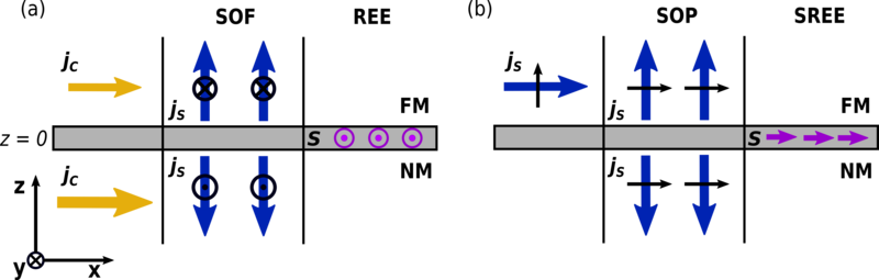
The first two terms in Eq. (5.34), along with the first four terms in Eqs. (5.34b) and (5.34c), represent out-of-plane charge and spin currents originating from the electrical potential and spin accumulation drops across the interface. These contributions account for the bulk out-of-plane currents in the NM and FM regions interacting with the interface, and are analogous to the interface currents described by the MCT. The fifth and sixth terms in Eqs. (5.34b) and (5.34c) describe out-of-plane spin currents induced by in-plane charge and spin currents, associated with the spin-orbit filtering (SOF) and spin-orbit precession (SOP) mechanisms, respectively [80]. The SOF mechanism arises because the interfacial SOC acts as a spin- and momentum-dependent filter, converting an initially unpolarized stream of electrons into a spin-polarized one through the interface scattering. In contrast, SOP occurs when a spin-polarized stream of electrons incident on the interface undergoes a change in polarization due to precession around the interfacial SOC field during scattering. The third and fourth terms in Eq. (5.34) describe the reciprocal effect, in which in-plane charge and spin currents generate out-of-plane charge currents.

The transmitted spin-polarized electron fluxes resulting from SOF and SOP also give rise to a non-equilibrium interfacial spin density. For a Rashba-type SOC, this interfacial spin density is analogous to the REE. Figure 5.1 illustrates the spin currents and interfacial spin densities produced when in-plane currents interact with the interfacial SOC in the Rashba SOC case with \(u_m = 0\). The spin density generated by SOF is oriented along \(\mathbf {E}\times \mathbf {z}\), consistent with standard 2D REE models, and is therefore identified with the REE. By contrast, the SOP-driven contribution is polarized along \((\mathbf {E}\times \mathbf {z})\times \mathbf {m}\). Since this polarization direction is distinct and the effect originates from the in-plane spin current of the FM layer, it will be referred to as the spin REE (SREE), distinguishing it from the conventional REE induced by in-plane charge currents. In the case of a Rashba-type SOC, the SOF, SOP, REE, and SREE will be collectively referred to as the Rashba Effect (RE).

5.3.3 Interfacial and Bulk Spin Torques

Equation (5.34) enforces continuity of the charge current across the interface, guaranteeing particle flux conservation. In contrast, the spin current is not conserved as interfacial scattering transfers part of the spin angular momentum to the effective field. This transfer can be expressed in terms of the non-equilibrium spin density generated at the interface by the incident in-plane and out-of-plane currents, which couples to the effective field via the interfacial exchange interaction. To satisfy total angular momentum conservation, the effective field at the interface must then experience a torque. At \(z=0\), only the transmitted contributions to the distribution remain, so the ensemble-averaged spin density at the interface is given by

\begin{equation} \label {eq:interfacial_spin_accumulation} \langle \bm {s}\rangle =\frac {-2m_e}{e\hbar A} \sum _{\bm {\bm {k_\|}}\in \mathrm {FS}} \frac {1}{k_z}\operatorname {Tr}\left [\bm {\hat {\sigma }}\left ( \mathcal {T}^{\uparrow \uparrow }_{\bm {k}}\hat {p}_{\bm {k}}^\uparrow \left (\hat {g}_{\bm {k}}^{\mathrm {N}} + \hat {g}_{\bm {k}}^{\mathrm {F}}\right )\hat {p}_{\bm {k}}^\uparrow +\mathcal {T}^{\downarrow \downarrow }_{\bm {k}}\hat {p}_{\bm {k}}^\downarrow \left (\hat {g}_{\bm {k}}^{\mathrm {N}} + \hat {g}_{\bm {k}}^{\mathrm {F}}\right )\hat {p}_{\bm {k}}^\downarrow +\mathcal {T}^{\uparrow \downarrow }_{\bm {k}}\hat {p}_{\bm {k}}^\uparrow \left (\hat {g}_{\bm {k}}^{\mathrm {N}} + \hat {g}_{\bm {k}}^{\mathrm {F}}\right )\hat {p}_{\bm {k}}^\downarrow +(\mathcal {T}^{\uparrow \downarrow }_{\bm {k}})^*\hat {p}_{\bm {k}}^\downarrow \left (\hat {g}_{\bm {k}}^{\mathrm {N}} + \hat {g}_{\bm {k}}^{\mathrm {F}}\right )\hat {p}_{\bm {k}}^\uparrow \right )\right ]. \end{equation}

When the effective field contains both a magnetic exchange and spin-orbit interaction, the resulting interfacial torque can be decomposed into two distinct contributions, each associated with one of these fields. The total torque transferred to the magnetization via the interfacial exchange interaction reads [75, 76]

\begin{equation} \label {eq:interface_torque_amin} \bm {\tau _s^\mathrm {mag}} = \frac {\mu _B}{e}\int _{0^-}^{0+}dz \frac {J_{m}}{\hbar }\delta (z)\left [\langle \bm {s}\rangle \times \bm {m}\right ]. \end{equation}

Inserting Eq. (5.37) into Eq. (5.38) and performing the trace yields

\begin{equation} \label {eq:interface_torque} \bm {\tau _s^\mathrm {mag}} = -\frac {\mu _B}{e}\left [ \left ( \tilde {\Gamma }^{\mathrm {mag}}_{+} - \tilde {\Gamma }^{\mathrm {mag}}_{\uparrow \downarrow }\right )\overline {\bm { V_{s}}} +\left (\bm {\gamma ^{\mathrm {mag},F}_{-}}+\bm {\gamma ^{\mathrm {mag},N}_{-}}\right )E_x +\beta _{\tau }\left (\tilde {\gamma }^{\mathrm {mag},F}_{+} - \tilde {\gamma }^{\mathrm {mag},F}_{\uparrow \downarrow } \right )\bm {m}E_x\right ], \end{equation}

where \(\overline {\bm { V_{s}}}=\bm { V^F_{s}}+\bm { V^N_{s}}\), and the interface torque conductances (torkances) and conductivities (torkivities) are given by the following expressions:

\begin{align} \begin{split} \tilde {\Gamma }^{\mathrm {mag},l}_{+} & = 2u_m\int \frac {d\bm {k_\|}}{(2\pi )^2}\left (\frac {k_x}{k_F}\right )^l\frac {k_F}{k_z} \left [\mathcal {T}^{\uparrow \uparrow }(\bm {k_\|}) + \mathcal {T}^{\downarrow \downarrow }(\bm {k_\|})\right ] \times [\bm {m}\times \bm {b}(\bm {k_\|})]\otimes \bm {b}(\bm {k_\|}), \end {split} \\ \begin{split} \tilde {\Gamma }^{\mathrm {mag},l}_{\uparrow \downarrow } & = 2u_m\int \frac {d\bm {k_\|}}{(2\pi )^2}\left (\frac {k_x}{k_F}\right )^l\frac {k_F}{k_z} [\bm {m}]_\times [\bm {b}(\bm {k_\|})]_\times \times \left (2\operatorname {Re}[\mathcal {T}^{\uparrow \downarrow }(\bm {k_\|})][\bm {b}(\bm {k_\|})]_\times - 2\operatorname {Im}[\mathcal {T}^{\uparrow \downarrow }(\bm {k_\|})]\right ), \end {split} \end{align}

\begin{align} \bm {\gamma ^{\mathrm {mag},F/N}_{-}} & = v_F\bm {\Gamma ^{\mathrm {mag},1}_{-}}\tau ^{F/N}, & \tilde {\gamma }^{\mathrm {mag},F/N}_{+} & = v_F\tilde {\Gamma }^{\mathrm {mag},1}_{+}\tau ^{F/N}, \nonumber \\ \tilde {\gamma }^{\mathrm {mag},F/N}_{\uparrow \downarrow } & = v_F\tilde {\Gamma }^{\mathrm {mag},1}_{\uparrow \downarrow }\tau ^{F/N}. & & \end{align} In Eq. (5.39), the first term represents the torque arising from transmitted out-of-plane spin currents. The second term corresponds to the REE spin density generated by in-plane charge currents at the interface, and the third term captures the spin SREE contribution originating from in-plane spin currents. The interfacial torque can be included in the LLG equation within a region near the interface with thickness \(d_h\) as follows \(\bm {T^\mathrm {int}_s} = \bm {\tau ^\mathrm {mag}_s/d_h}\).

The torque acting on the spin-orbit component of the effective field reflects the transfer of angular momentum from the spin current to the crystal lattice, mediated by spin-orbit and Coulomb interactions [76]. This lattice torque is given by the remaining spin current not absorbed by the magnetization [76]:

\begin{equation} \bm {\tau _s^\mathrm {latt}} = \Delta \bm {J_{zs}} - \bm {\tau _s^\mathrm {mag}}. \end{equation}

Beyond the interfacial contributions, the magnetization within the FM bulk also experiences torques arising from transverse spin currents. As these transverse spin currents propagate in the FM, they transfer angular momentum to the magnetization, giving rise to STTs. If the transverse spin currents are assumed to decay completely inside the bulk, the total torque acting on the magnetization is simply given by the transverse spin current at the FM side of the interface: \(\bm {\tau _s^\mathrm {FM}} = (I-\bm {m}\otimes \bm {m})\bm {J_{zs}}(0^+)\). In contrast, if the FM layer is sufficiently thin such that the transverse spin currents do not fully relax, the bulk torque must instead be evaluated from the net loss of transverse spin current across the FM layer, which is obtained by integrating Eq. (4.19) over the volume of the FM layer.

The total torque can be divided into five different contributions: \(\bm {\tau ^\mathrm {tot}} = \bm {\tau ^\mathrm {MCT}_{\mu }} + \bm {\tau ^\mathrm {SOF}_E} + \bm {\tau ^\mathrm {SOP}_E} + \bm {\tau ^\mathrm {REE}_E} + \bm {\tau ^\mathrm {SREE}_E}\). The first contribution \(\bm {\tau ^\mathrm {MCT}_{\mu }}\) describes the torque from the out-of-plane spin currents contributing to the spin accumulation at the interface and the transverse spin current in the FM layer, such as the SHE current, which is captured by the spin potentials at either side of the interface. This contribution is analogous to the torque from the MCT, which has been modified by the interfacial SOC:

\begin{equation} \label {eq:tau_mu} \bm {\tau ^\mathrm {MCT}_{\mu }} = -\frac {\mu _B}{e} \left (\tilde {\Gamma }^{\mathrm {mag}}_{+}-\tilde {\Gamma }^{\mathrm {mag}}_{\uparrow \downarrow }\right )\overline {\bm { V_{s}}} + \frac {\mu _B}{e}(I-\bm {m}\otimes \bm {m})\big (\tilde {G}_{+}\Delta \bm { V_{s}}+\bm {G_{-}}\Delta V_{c} + \tilde {G}_{\uparrow \downarrow }\bm { V_{s}^{\mathrm {N}}} - \tilde {\Gamma }_{\uparrow \downarrow }\bm { V_{s}^{\mathrm {F}}}\big ). \end{equation}

The remaining four contributions arise from the in-plane charge and spin currents on both sides of the interface. The first two correspond to the transverse spin currents on the FM side generated via SOF and SOP, which are expressed as

\begin{equation} \bm {\tau ^\mathrm {SOF}_E} = \frac {\mu _B}{e}(I-\bm {m}\otimes \bm {m})(\Delta \bm {\sigma _{-}}E_x), \end{equation}

and

\begin{equation} \bm {\tau ^\mathrm {SOP}_E} = \frac {\mu _B}{e}(I-\bm {m}\otimes \bm {m})[\beta _{\tau }(\tilde {\sigma }^F_{+}-\tilde {\sigma }^F_{\uparrow \downarrow })\bm {m}E_x], \end{equation}

respectively. The last two contributions arise from the REE and SREE-generated spin density at the interface, given by

\begin{equation} \bm {\tau ^\mathrm {REE}_E} = -\frac {\mu _B}{e}\left (\bm {\gamma ^{\mathrm {mag},F}_{-}}+\bm {\gamma ^{\mathrm {mag},N}_{-}}\right )E_x, \end{equation}

and

\begin{equation} \bm {\tau ^\mathrm {SREE}_E} = -\frac {\mu _B}{e}\beta _{\tau }\left (\tilde {\gamma }^{\mathrm {mag},F}_{+}-\tilde {\gamma }^{\mathrm {mag},F}_{\uparrow \downarrow } \right )\bm {m}E_x, \end{equation}

respectively.

5.3.4 Vanishing Interfacial Spin-Orbit Coupling Limit

In the limit of vanishing SOC: \(\bm {b}(\bm {k_\|}) = \bm {m}\) and \(u_{\bm {k}}^{\uparrow /\downarrow } = u_0 \mp u_m\). As both the effective field and the reduced conductances are even in \(\bm {k_\|}\), all the conductivities describing the shift of the Fermi sphere in Eqs. (5.34) and (5.39) vanish after integration due to the additional odd \(k_x/k_F\) factor in the Fermi surface integrals. Since the magnetic field at the interface is momentum-independent, it can be taken out of the Fermi surface integrals in (5.35), and the currents can be described in terms of scalar conductances:

\begin{equation} j_{zc}(0^{\mathbin {\textpm }}) = (G_{\uparrow \uparrow } + G_{\downarrow \downarrow })\Delta V_{c} + (G_{\uparrow \uparrow } - G_{\downarrow \downarrow })\Delta \bm { V_{s}}\cdot \bm {m}, \end{equation}

\begin{multline} \bm {J_{zs}}(0^+) = \frac {\mu _B}{e}\left [ (G_{\uparrow \uparrow } - G_{\downarrow \downarrow })\Delta V_{c}\bm {m} +(G_{\uparrow \uparrow } + G_{\downarrow \downarrow })\bm {m}(\Delta \bm { V_{s}}\cdot \bm {m}) + 2\operatorname {Re}\{G_{\uparrow \downarrow }\}\bm {m}\times (\bm { V_{s}^{\mathrm {F}}}\times \bm {m}) - 2\operatorname {Im}\{G_{\uparrow \downarrow }\}\bm { V_{s}^{\mathrm {F}}\times \bm {m}} \right . \\ \left . - 2\operatorname {Re}\{\Gamma _{\uparrow \downarrow }\}\bm {m}\times (\bm { V_{s}^{\mathrm {N}}}\times \bm {m}) + 2\operatorname {Im}\{\Gamma _{\uparrow \downarrow }\}\bm { V_{s}^{\mathrm {N}}\times \bm {m}} \right ], \end{multline}

\begin{multline} \bm {J_{zs}}(0^-) = \frac {\mu _B}{e}\left [ (G_{\uparrow \uparrow } - G_{\downarrow \downarrow })\Delta V_{c}\bm {m} +(G_{\uparrow \uparrow } + G_{\downarrow \downarrow })\bm {m}(\Delta \bm { V_{s}}\cdot \bm {m}) - 2\operatorname {Re}\{G_{\uparrow \downarrow }\}\bm {m}\times (\bm { V_{s}^{\mathrm {N}}}\times \bm {m}) + 2\operatorname {Im}\{G_{\uparrow \downarrow }\}\bm { V_{s}^{\mathrm {N}}\times \bm {m}} \right . \\ \left . + 2\operatorname {Re}\{\Gamma _{\uparrow \downarrow }\}\bm {m}\times (\bm { V_{s}^{\mathrm {F}}}\times \bm {m}) - 2\operatorname {Im}\{\Gamma _{\uparrow \downarrow }\}\bm { V_{s}^{\mathrm {F}}\times \bm {m}}\right ]. \end{multline} The scalar interface conductances are given by the Fermi surface integrals

\begin{equation} \label {eq:scalar_conductances_um} G_{ss^\prime } = \int \frac {d\bm {k_\|}}{(2\pi )^2}\mathcal {G}^{ss^\prime }(\bm {k_\|}), \text { and } \quad \Gamma _{ss^\prime } = \int \frac {d\bm {k_\|}}{(2\pi )^2}\mathcal {T}^{ss^\prime }(\bm {k_\|}), \end{equation}

for \(s,s^\prime \in \{\uparrow ,\downarrow \}\). The currents in Eq. (5.48) are almost identical to the ones from the MCT except for including a transmission spin-mixing conductance \(\Gamma _{\uparrow \downarrow }\) which accounts for the transverse spin components in the FM layer that are often ignored as the spin dephasing length is typically much smaller compared to the FM layer thickness. Assuming the transverse spin accumulation quickly dephases (\(\lambda _\phi \to 0\) ) in the bulk of the FM layer, then \(\bm { V^F_s} \to V^F_s\bm {m}\) and \(\bm {J_{zs}}(0^+) \to {J_{zs}}(0^+)\bm {m}\). In this limit, the expressions for the interface currents from the MCT are recovered.

Without SOC, the lattice torque is no longer present, and only the interface torque acting on the magnetization is present, which reduces to

\begin{gather} \bm {\tau _s^\mathrm {mag}} = \frac {2\mu _B}{e}\left [\operatorname {Im}\{\Gamma ^\mathrm {mag}_{\uparrow \downarrow }\}\bm {m}\times (\bm {m}\times \overline {\bm { V_{s}}}) +\operatorname {Re}\{\Gamma ^\mathrm {mag}_{\uparrow \downarrow }\}\bm {m}\times \overline {\bm { V_{s}}}\right ], \end{gather} where the torque is given by the Fermi surface integral

\begin{equation} \label {eq:scalar_torkance} \Gamma ^\mathrm {mag}_{\uparrow \downarrow } = 2u_m \int \frac {d\bm {k_\|}}{(2\pi )^2}\frac {k_F}{k_z}\mathcal {T}^{\uparrow \downarrow }(\bm {k_\|}). \end{equation}

The difference in spin currents across the interface is given by

\begin{equation} \Delta \bm {J_{zs}} = \bm {J_{zs}}(0^-) - \bm {J_{zs}}(0^+) = \frac {2\mu _B}{e}\left [\left (\operatorname {Re}\{G_{\uparrow \downarrow }\}-\operatorname {Re}\{\Gamma _{\uparrow \downarrow }\}\right )\bm {m}\times \left (\bm {m}\times \overline {\bm { V_{s}}}\right ) - \left (\operatorname {Im}\{G_{\uparrow \downarrow }\}-\operatorname {Im}\{\Gamma _{\uparrow \downarrow }\}\right )\bm {m}\times \overline {\bm { V_{s}}}\right ]. \end{equation}

With some algebra, it can be shown that \(\operatorname {Re}\{G_{\uparrow \downarrow }\}- \operatorname {Re}\{\Gamma _{\uparrow \downarrow }\} = \operatorname {Im}\{\Gamma ^\mathrm {mag}_{\uparrow \downarrow }\}\) and \(\operatorname {Im}\{G_{\uparrow \downarrow }\}- \operatorname {Im}\{\Gamma _{\uparrow \downarrow }\} = -\operatorname {Re}\{\Gamma ^\mathrm {mag}_{\uparrow \downarrow }\}\), i.e., the interfacial torque is exactly given by the drop of spin current across the interface. Using these identities, the total torque acting on the magnetization of the FM layer is then given by the sum of the interfacial torque and the transverse spin current at the FM side of the interface:

\begin{multline} \label {eq:torque_rashba} \bm {\tau ^\mathrm {tot}} = \bm {\tau ^\mathrm {mag}} + \bm {\tau ^\mathrm {FM}} = \frac {2\mu _B}{e}\left [(\operatorname {Im}\{\Gamma ^\mathrm {mag}_{\uparrow \downarrow }\}- \operatorname {Re}\{G_{\uparrow \downarrow }\})\bm {m}\times (\bm {m}\times \bm { V_{s}^{\mathrm {F}}}) + (\operatorname {Re}\{\Gamma ^\mathrm {mag}_{\uparrow \downarrow }\}+ \operatorname {Im}\{G_{\uparrow \downarrow }\})\bm {m}\times \bm { V_{s}^{\mathrm {F}}} \right . \\ \left . + (\operatorname {Im}\{\Gamma ^\mathrm {mag}_{\uparrow \downarrow }\} + \operatorname {Re}\{\Gamma _{\uparrow \downarrow }\})\bm {m}\times (\bm {m}\times \bm { V_{s}^{\mathrm {N}}}) + (\operatorname {Re}\{\Gamma ^\mathrm {mag}_{\uparrow \downarrow }\} - \operatorname {Im}\{\Gamma _{\uparrow \downarrow }\})\bm {m}\times \bm { V_{s}^{\mathrm {N}}}\right ] \\ = \frac {2\mu _B}{e}\left [\operatorname {Re}\{G_{\uparrow \downarrow }\}\bm {m}\times (\bm {m}\times \bm { V_{s}^{\mathrm {N}}}) - \operatorname {Im}\{G_{\uparrow \downarrow }\}\bm {m}\times \bm { V_{s}^{\mathrm {N}}} - \operatorname {Re}\{\Gamma _{\uparrow \downarrow }\}\bm {m}\times (\bm {m}\times \bm { V_{s}^{\mathrm {F}}}) + \operatorname {Im}\{\Gamma _{\uparrow \downarrow }\}\bm {m}\times \bm { V_{s}^{\mathrm {F}}}\right ], \end{multline} which is exactly the transverse spin current on the NM side of the interface. Assuming \(\bm { V_{s}^{\mathrm {F}}} \| \bm {m}\), Eq. (5.53) reduces to the spin torque from the MCT. Supposing the spin current in the bulk of the NM layer is entirely due to the SHE, one can approximate \(\bm { V^N_s} \approx (\bm {\hat {E}}\times \bm {\hat {z}}) V^N_s\), then the ratio between the typical DL and FL terms are described by the real and imaginary parts of the spin-mixing conductance, respectively.

5.3.5 Vanishing Interfacial Exchange Interaction Limit

Considering the limit case of a vanishing interfacial exchange interaction and a strong Rashba SOC at the interface. The direction of the effective field is given by \(\bm {b}(\bm {k_\|}) = \bm {k}\times \bm {z}/\|\bm {k}\times \bm {z}\|\). The dimensionless majority/minority spin potential barriers are given by \(u^{\uparrow /\downarrow } = u_0\mp u_R\|\bm {\hat {k}}\times \bm {\hat {z}}\|\), where \(u_R\) is the dimensionless magnitude of the Rashba interaction at the interface. In this regime, the reduced conductances are again even in \(\bm {k_\|}\); however, since the effective field is odd in \(\bm {k_\|}\), the currents simplify to the following expressions:

\begin{equation} j_{zc}(0^{\mathbin {\textpm }}) = (G_{\uparrow \uparrow } + G_{\downarrow \downarrow })\Delta V_{c} + \beta _{\tau }(\sigma ^F_{\uparrow \uparrow }-\sigma ^F_{\downarrow \downarrow })(\bm {E}\times \bm {\hat {z}})\cdot \bm {m}, \end{equation}

\begin{equation} \bm {J_{zs}}(0^+) = \frac {\mu _B}{e}\left [(G_{\uparrow \uparrow } + G_{\downarrow \downarrow })\bm {\hat {z}}\times (\Delta \bm { V_{s}}\times \bm {\hat {z}}) + 2\operatorname {Re}\{G_{\uparrow \downarrow }\}[\bm {\hat {z}}(\bm {\hat {z}}\cdot \bm { V_{s}^{\mathrm {F}}})] - 2\operatorname {Re}\{\Gamma _{\uparrow \downarrow }\}[\bm {\hat {z}}(\bm {\hat {z}}\cdot \bm { V_{s}^{\mathrm {N}}})] + (\Delta \sigma _{\uparrow \uparrow }-\Delta \sigma _{\downarrow \downarrow })(\bm {E}\times \bm {\hat {z}}) + 2\beta _{\tau }\operatorname {Im}\{\sigma ^F_{\uparrow \downarrow }\}(\bm {E}\times \bm {\hat {z}})\times \bm {m}\right ], \end{equation}

\begin{equation} \bm {J_{zs}}(0^-) = \frac {\mu _B}{e}\left [(G_{\uparrow \uparrow } + G_{\downarrow \downarrow })\bm {\hat {z}}\times (\Delta \bm { V_{s}}\times \bm {\hat {z}}) - 2\operatorname {Re}\{G_{\uparrow \downarrow }\}\bm {\hat {z}}(\bm {\hat {z}}\cdot \bm { V_{s}^{\mathrm {N}}}) + 2\operatorname {Re}\{\Gamma _{\uparrow \downarrow }\}\bm {\hat {z}}(\bm {\hat {z}}\cdot \bm { V_{s}^{\mathrm {F}}}) + (\Delta \sigma _{\uparrow \uparrow }-\Delta \sigma _{\downarrow \downarrow })(\bm {E}\times \bm {\hat {z}}) + 2\beta _{\tau }\operatorname {Im}\{\gamma ^F_{\uparrow \downarrow }\}(\bm {E}\times \bm {\hat {z}})\times \bm {m}\right ], \end{equation}

where \(\bm {E} = E_x\bm {\hat {x}}\) is the electric field along \(x\). The scalar interface conductances and conductivities are defined as follows:

\begin{align} \label {eq:scalar_conductances_uR} G_{ss^\prime } & = \int \frac {d\bm {k_\|}}{(2\pi )^2}\mathcal {G}^{ss^\prime }(\bm {k_\|})\frac {k^2_x}{k^2_x + k^2_y}, \\ \Gamma _{ss^\prime } & = \int \frac {d\bm {k_\|}}{(2\pi )^2}\mathcal {T}^{ss^\prime }(\bm {k_\|})\frac {k^2_x}{k^2_x + k^2_y}, \\ \sigma ^{F/N}_{ss^\prime } & = v_F\tau ^{F/N} \int \frac {d\bm {k_\|}}{(2\pi )^2}\mathcal {G}^{ss^\prime }(\bm {k_\|})\frac {k^2_x}{\sqrt {k^2_x + k^2_y}}, \\ \gamma ^{F/N}_{ss^\prime } & = v_F\tau ^{F/N} \int \frac {d\bm {k_\|}}{(2\pi )^2}\mathcal {T}^{ss^\prime }(\bm {k_\|})\frac {k^2_x}{\sqrt {k^2_x + k^2_y}} , \end{align} for \(s,s^\prime \in \{\uparrow ,\downarrow \}\). In this regime, the conductance terms coupled to the charge and spin potentials are described in terms of the interface normal instead of the magnetization direction. The last two terms are again the SOF and SOP currents, respectively. The SOF current polarization direction is along the momentum-averaged field that the in-plane current experiences, which is given by the cross product \((\bm {E}\times \bm {\hat {z}})\). In contrast, the SOP field is given by the precession of the in-plane FM current polarized along \(\bm {m}\) around this field, described by the cross products \((\bm {E}\times \bm {\hat {z}})\times \bm {m}\).

With \(u_m = 0\), there is no torque acting on the magnetization at the interface; instead, the difference in spin current across the interface is entirely lost to the lattice, and one obtains

\begin{equation} \bm {\tau _s^\mathrm {latt}} = \Delta \bm {J_{zs}} = \frac {2\mu _B}{e}(\operatorname {Re}\{G_{\uparrow \downarrow }\}- \operatorname {Re}\{\Gamma _{\uparrow \downarrow }\})\bm {\hat {z}}( \bm {\hat {z}}\cdot \overline {\bm { V_{s}}}) + \frac {2\mu _B}{e}\beta _{\tau }(\operatorname {Im}\{\gamma ^{F}_{\uparrow \downarrow }\} -\operatorname {Im}\{\sigma ^{F}_{\uparrow \downarrow }\} ) (\bm {E}\times \bm {\hat {z}})\times \bm {m}. \end{equation}

Assuming the transverse spin current fully decays in the bulk, the total torque on the magnetization is given by the transverse spin current in the FM layer:

\begin{multline} \label {eq:total_rashba_torque} \bm {\tau _s^\mathrm {tot}} = (1-\bm {m}\otimes \bm {m})\bm {\tau _s^{FM}} = \frac {\mu _B}{e}\left [ (G_{\uparrow \uparrow } + G_{\downarrow \downarrow })\bm {m}\times \left \{\left [\bm {\hat {z}}\times \left (\Delta \bm { V_{s}}\times \bm {\hat {z}}\right )\right ]\times \bm {m}\right \} \right .\\ \left . +2\operatorname {Re}\{G_{\uparrow \downarrow }\}\bm {m}\times \left (\bm {\hat {z}}\times \bm {m}\right )\left (\bm {\hat {z}}\cdot \bm { V_{s}^{\mathrm {F}}}\right ) -2\operatorname {Re}\{\Gamma _{\uparrow \downarrow }\}\bm {m}\times \left (\bm {\hat {z}}\times \bm {m}\right )\left (\bm {\hat {z}}\cdot \bm { V_{s}^{\mathrm {N}}}\right ) \right .\\ \left . +(\Delta \sigma _{\uparrow \uparrow }-\Delta \sigma _{\downarrow \downarrow })\bm {m}\times [(\bm {E}\times \bm {\hat {z}})\times \bm {m}] +2\beta _{\tau }\operatorname {Im}\{\sigma ^\mathrm {F}_{\uparrow \downarrow }\}(\bm {E}\times \bm {\hat {z}})\times \bm {m}\right ]. \end{multline} Assuming the out-of-plane spin current from the NM impinging on the interface is generated by the SHE and that the transverse spin current rapidly dephases in the FM layer \(\bm { V^N_s} \approx (\bm {\hat {E}}\times \bm {\hat {z}}) V^N_s\) and \(\bm { V^F_s} \approx \bm {m} V^F_s\). The total torque then reads

\begin{multline} \label {eq:total_rashba_torque_approx} \bm {\tau _s^\mathrm {tot}} = (G_{\uparrow \uparrow } + G_{\downarrow \downarrow })\bm {m}\times \left [(\bm {\hat {E}}\times \bm {\hat {z}})\times \bm {m}\right ] V^N_{s} (2\operatorname {Re}\{G_{\uparrow \downarrow }\}-G_{\uparrow \uparrow } - G_{\downarrow \downarrow })\bm {m}\times (\bm {\hat {z}}\times \bm {m})(\bm {\hat {z}}\cdot \bm {m}) V^F_{s} \\ +(\Delta \sigma _{\uparrow \uparrow }-\Delta \sigma _{\downarrow \downarrow })\bm {m}\times \left [(\bm {E}\times \bm {\hat {z}})\times \bm {m}\right ] +2\beta _{\tau }\operatorname {Im}\{\sigma ^\mathrm {F}_{\uparrow \downarrow }\}(\bm {E}\times \bm {\hat {z}})\times \bm {m}. \end{multline} The second term describes a new contribution to the torque, which damps the magnetization towards \(\bm {\hat {z}}\) and vanishes when \(\bm {m}\) is in the plane; the first and third term describes the typical DL torque, while the last term describes the typical FL torque. The new torque term originates from the longitudinal out-of-plane currents in the FM interacting with the interface and could potentially facilitate switching of perpendicular magnetic states.