(image) (image) [ Previous ] [ Home ] [ Next ]

Modeling Spin-Orbit Torques
in Advanced Magnetoresistive Devices

\(\newcommand{\footnotename}{footnote}\) \(\def \LWRfootnote {1}\) \(\newcommand {\footnote }[2][\LWRfootnote ]{{}^{\mathrm {#1}}}\) \(\newcommand {\footnotemark }[1][\LWRfootnote ]{{}^{\mathrm {#1}}}\) \(\let \LWRorighspace \hspace \) \(\renewcommand {\hspace }{\ifstar \LWRorighspace \LWRorighspace }\) \(\newcommand {\mathnormal }[1]{{#1}}\) \(\newcommand \ensuremath [1]{#1}\) \(\newcommand {\LWRframebox }[2][]{\fbox {#2}} \newcommand {\framebox }[1][]{\LWRframebox } \) \(\newcommand {\setlength }[2]{}\) \(\newcommand {\addtolength }[2]{}\) \(\newcommand {\setcounter }[2]{}\) \(\newcommand {\addtocounter }[2]{}\) \(\newcommand {\arabic }[1]{}\) \(\newcommand {\number }[1]{}\) \(\newcommand {\noalign }[1]{\text {#1}\notag \\}\) \(\newcommand {\cline }[1]{}\) \(\newcommand {\directlua }[1]{\text {(directlua)}}\) \(\newcommand {\luatexdirectlua }[1]{\text {(directlua)}}\) \(\newcommand {\protect }{}\) \(\def \LWRabsorbnumber #1 {}\) \(\def \LWRabsorbquotenumber "#1 {}\) \(\newcommand {\LWRabsorboption }[1][]{}\) \(\newcommand {\LWRabsorbtwooptions }[1][]{\LWRabsorboption }\) \(\def \mathchar {\ifnextchar "\LWRabsorbquotenumber \LWRabsorbnumber }\) \(\def \mathcode #1={\mathchar }\) \(\let \delcode \mathcode \) \(\let \delimiter \mathchar \) \(\def \oe {\unicode {x0153}}\) \(\def \OE {\unicode {x0152}}\) \(\def \ae {\unicode {x00E6}}\) \(\def \AE {\unicode {x00C6}}\) \(\def \aa {\unicode {x00E5}}\) \(\def \AA {\unicode {x00C5}}\) \(\def \o {\unicode {x00F8}}\) \(\def \O {\unicode {x00D8}}\) \(\def \l {\unicode {x0142}}\) \(\def \L {\unicode {x0141}}\) \(\def \ss {\unicode {x00DF}}\) \(\def \SS {\unicode {x1E9E}}\) \(\def \dag {\unicode {x2020}}\) \(\def \ddag {\unicode {x2021}}\) \(\def \P {\unicode {x00B6}}\) \(\def \copyright {\unicode {x00A9}}\) \(\def \pounds {\unicode {x00A3}}\) \(\let \LWRref \ref \) \(\renewcommand {\ref }{\ifstar \LWRref \LWRref }\) \( \newcommand {\multicolumn }[3]{#3}\) \(\require {textcomp}\) \(\newcommand {\mathlarger }[1]{#1}\) \(\newcommand {\mathsmaller }[1]{#1}\) \(\newcommand {\intertext }[1]{\text {#1}\notag \\}\) \(\let \Hat \hat \) \(\let \Check \check \) \(\let \Tilde \tilde \) \(\let \Acute \acute \) \(\let \Grave \grave \) \(\let \Dot \dot \) \(\let \Ddot \ddot \) \(\let \Breve \breve \) \(\let \Bar \bar \) \(\let \Vec \vec \) \(\newcommand {\bm }[1]{\boldsymbol {#1}}\) \(\require {mathtools}\) \(\newenvironment {crampedsubarray}[1]{}{}\) \(\newcommand {\smashoperator }[2][]{#2\limits }\) \(\newcommand {\SwapAboveDisplaySkip }{}\) \(\newcommand {\LaTeXunderbrace }[1]{\underbrace {#1}}\) \(\newcommand {\LaTeXoverbrace }[1]{\overbrace {#1}}\) \(\newcommand {\LWRmultlined }[1][]{\begin {multline*}}\) \(\newenvironment {multlined}[1][]{\LWRmultlined }{\end {multline*}}\) \(\let \LWRorigshoveleft \shoveleft \) \(\renewcommand {\shoveleft }[1][]{\LWRorigshoveleft }\) \(\let \LWRorigshoveright \shoveright \) \(\renewcommand {\shoveright }[1][]{\LWRorigshoveright }\) \(\newcommand {\shortintertext }[1]{\text {#1}\notag \\}\) \(\newcommand {\vcentcolon }{\mathrel {\unicode {x2236}}}\) \(\newcommand {\tothe }[1]{^{#1}}\) \(\newcommand {\raiseto }[2]{{#2}^{#1}}\) \(\newcommand {\LWRsiunitxEND }{}\) \(\def \LWRsiunitxang #1;#2;#3;#4\LWRsiunitxEND {\ifblank {#1}{}{\num {#1}\degree }\ifblank {#2}{}{\num {#2}^{\unicode {x2032}}}\ifblank {#3}{}{\num {#3}^{\unicode {x2033}}}}\) \(\newcommand {\ang }[2][]{\LWRsiunitxang #2;;;\LWRsiunitxEND }\) \(\def \LWRsiunitxdistribunit {}\) \(\newcommand {\LWRsiunitxENDTWO }{}\) \(\def \LWRsiunitxprintdecimalsubtwo #1,#2,#3\LWRsiunitxENDTWO {\ifblank {#1}{0}{\mathrm {#1}}\ifblank {#2}{}{{\LWRsiunitxdecimal }\mathrm {#2}}}\) \(\def \LWRsiunitxprintdecimalsub #1.#2.#3\LWRsiunitxEND {\LWRsiunitxprintdecimalsubtwo #1,,\LWRsiunitxENDTWO \ifblank {#2}{}{{\LWRsiunitxdecimal }\LWRsiunitxprintdecimalsubtwo #2,,\LWRsiunitxENDTWO }}\) \(\newcommand {\LWRsiunitxprintdecimal }[1]{\LWRsiunitxprintdecimalsub #1...\LWRsiunitxEND }\) \(\def \LWRsiunitxnumplus #1+#2+#3\LWRsiunitxEND {\ifblank {#2}{\LWRsiunitxprintdecimal {#1}}{\ifblank {#1}{\LWRsiunitxprintdecimal {#2}}{\LWRsiunitxprintdecimal {#1}\unicode {x02B}\LWRsiunitxprintdecimal {#2}}}\LWRsiunitxdistribunit }\) \(\def \LWRsiunitxnumminus #1-#2-#3\LWRsiunitxEND {\ifblank {#2}{\LWRsiunitxnumplus #1+++\LWRsiunitxEND }{\ifblank {#1}{}{\LWRsiunitxprintdecimal {#1}}\unicode {x02212}\LWRsiunitxprintdecimal {#2}\LWRsiunitxdistribunit }}\) \(\def \LWRsiunitxnumpmmacro #1\pm #2\pm #3\LWRsiunitxEND {\ifblank {#2}{\LWRsiunitxnumminus #1---\LWRsiunitxEND }{\LWRsiunitxprintdecimal {#1}\unicode {x0B1}\LWRsiunitxprintdecimal {#2}\LWRsiunitxdistribunit }}\) \(\def \LWRsiunitxnumpm #1+-#2+-#3\LWRsiunitxEND {\ifblank {#2}{\LWRsiunitxnumpmmacro #1\pm \pm \pm \LWRsiunitxEND }{\LWRsiunitxprintdecimal {#1}\unicode {x0B1}\LWRsiunitxprintdecimal {#2}\LWRsiunitxdistribunit }}\) \(\newcommand {\LWRsiunitxnumscientific }[2]{\ifblank {#1}{}{\ifstrequal {#1}{-}{-}{\LWRsiunitxprintdecimal {#1}\times }}10^{\LWRsiunitxprintdecimal {#2}}\LWRsiunitxdistribunit }\) \(\def \LWRsiunitxnumD #1D#2D#3\LWRsiunitxEND {\ifblank {#2}{\LWRsiunitxnumpm #1+-+-\LWRsiunitxEND }{\mathrm {\LWRsiunitxnumscientific {#1}{#2}}}}\) \(\def \LWRsiunitxnumd #1d#2d#3\LWRsiunitxEND {\ifblank {#2}{\LWRsiunitxnumD #1DDD\LWRsiunitxEND }{\mathrm {\LWRsiunitxnumscientific {#1}{#2}}}}\) \(\def \LWRsiunitxnumE #1E#2E#3\LWRsiunitxEND {\ifblank {#2}{\LWRsiunitxnumd #1ddd\LWRsiunitxEND }{\mathrm {\LWRsiunitxnumscientific {#1}{#2}}}}\) \(\def \LWRsiunitxnume #1e#2e#3\LWRsiunitxEND {\ifblank {#2}{\LWRsiunitxnumE #1EEE\LWRsiunitxEND }{\mathrm {\LWRsiunitxnumscientific {#1}{#2}}}}\) \(\def \LWRsiunitxnumx #1x#2x#3x#4\LWRsiunitxEND {\ifblank {#2}{\LWRsiunitxnume #1eee\LWRsiunitxEND }{\ifblank {#3}{\LWRsiunitxnume #1eee\LWRsiunitxEND \times \LWRsiunitxnume #2eee\LWRsiunitxEND }{\LWRsiunitxnume #1eee\LWRsiunitxEND \times \LWRsiunitxnume #2eee\LWRsiunitxEND \times \LWRsiunitxnume #3eee\LWRsiunitxEND }}}\) \(\newcommand {\num }[2][]{\LWRsiunitxnumx #2xxxxx\LWRsiunitxEND }\) \(\newcommand {\si }[2][]{\mathrm {\gsubstitute {#2}{~}{\,}}}\) \(\def \LWRsiunitxSIopt #1[#2]#3{\def \LWRsiunitxdistribunit {\,\si {#3}}{#2}\num {#1}\def \LWRsiunitxdistribunit {}}\) \(\newcommand {\LWRsiunitxSI }[2]{\def \LWRsiunitxdistribunit {\,\si {#2}}\num {#1}\def \LWRsiunitxdistribunit {}}\) \(\newcommand {\SI }[2][]{\ifnextchar [{\LWRsiunitxSIopt {#2}}{\LWRsiunitxSI {#2}}}\) \(\newcommand {\numlist }[2][]{\text {#2}}\) \(\newcommand {\numrange }[3][]{\num {#2}\ \LWRsiunitxrangephrase \ \num {#3}}\) \(\newcommand {\SIlist }[3][]{\text {#2}\,\si {#3}}\) \(\newcommand {\SIrange }[4][]{\num {#2}\,#4\ \LWRsiunitxrangephrase \ \num {#3}\,#4}\) \(\newcommand {\tablenum }[2][]{\mathrm {#2}}\) \(\newcommand {\ampere }{\mathrm {A}}\) \(\newcommand {\candela }{\mathrm {cd}}\) \(\newcommand {\kelvin }{\mathrm {K}}\) \(\newcommand {\kilogram }{\mathrm {kg}}\) \(\newcommand {\metre }{\mathrm {m}}\) \(\newcommand {\mole }{\mathrm {mol}}\) \(\newcommand {\second }{\mathrm {s}}\) \(\newcommand {\becquerel }{\mathrm {Bq}}\) \(\newcommand {\degreeCelsius }{\unicode {x2103}}\) \(\newcommand {\coulomb }{\mathrm {C}}\) \(\newcommand {\farad }{\mathrm {F}}\) \(\newcommand {\gray }{\mathrm {Gy}}\) \(\newcommand {\hertz }{\mathrm {Hz}}\) \(\newcommand {\henry }{\mathrm {H}}\) \(\newcommand {\joule }{\mathrm {J}}\) \(\newcommand {\katal }{\mathrm {kat}}\) \(\newcommand {\lumen }{\mathrm {lm}}\) \(\newcommand {\lux }{\mathrm {lx}}\) \(\newcommand {\newton }{\mathrm {N}}\) \(\newcommand {\ohm }{\mathrm {\Omega }}\) \(\newcommand {\pascal }{\mathrm {Pa}}\) \(\newcommand {\radian }{\mathrm {rad}}\) \(\newcommand {\siemens }{\mathrm {S}}\) \(\newcommand {\sievert }{\mathrm {Sv}}\) \(\newcommand {\steradian }{\mathrm {sr}}\) \(\newcommand {\tesla }{\mathrm {T}}\) \(\newcommand {\volt }{\mathrm {V}}\) \(\newcommand {\watt }{\mathrm {W}}\) \(\newcommand {\weber }{\mathrm {Wb}}\) \(\newcommand {\day }{\mathrm {d}}\) \(\newcommand {\degree }{\mathrm {^\circ }}\) \(\newcommand {\hectare }{\mathrm {ha}}\) \(\newcommand {\hour }{\mathrm {h}}\) \(\newcommand {\litre }{\mathrm {l}}\) \(\newcommand {\liter }{\mathrm {L}}\) \(\newcommand {\arcminute }{^\prime }\) \(\newcommand {\minute }{\mathrm {min}}\) \(\newcommand {\arcsecond }{^{\prime \prime }}\) \(\newcommand {\tonne }{\mathrm {t}}\) \(\newcommand {\astronomicalunit }{au}\) \(\newcommand {\atomicmassunit }{u}\) \(\newcommand {\bohr }{\mathit {a}_0}\) \(\newcommand {\clight }{\mathit {c}_0}\) \(\newcommand {\dalton }{\mathrm {D}_\mathrm {a}}\) \(\newcommand {\electronmass }{\mathit {m}_{\mathrm {e}}}\) \(\newcommand {\electronvolt }{\mathrm {eV}}\) \(\newcommand {\elementarycharge }{\mathit {e}}\) \(\newcommand {\hartree }{\mathit {E}_{\mathrm {h}}}\) \(\newcommand {\planckbar }{\mathit {\unicode {x210F}}}\) \(\newcommand {\angstrom }{\mathrm {\unicode {x212B}}}\) \(\let \LWRorigbar \bar \) \(\newcommand {\bar }{\mathrm {bar}}\) \(\newcommand {\barn }{\mathrm {b}}\) \(\newcommand {\bel }{\mathrm {B}}\) \(\newcommand {\decibel }{\mathrm {dB}}\) \(\newcommand {\knot }{\mathrm {kn}}\) \(\newcommand {\mmHg }{\mathrm {mmHg}}\) \(\newcommand {\nauticalmile }{\mathrm {M}}\) \(\newcommand {\neper }{\mathrm {Np}}\) \(\newcommand {\yocto }{\mathrm {y}}\) \(\newcommand {\zepto }{\mathrm {z}}\) \(\newcommand {\atto }{\mathrm {a}}\) \(\newcommand {\femto }{\mathrm {f}}\) \(\newcommand {\pico }{\mathrm {p}}\) \(\newcommand {\nano }{\mathrm {n}}\) \(\newcommand {\micro }{\mathrm {\unicode {x00B5}}}\) \(\newcommand {\milli }{\mathrm {m}}\) \(\newcommand {\centi }{\mathrm {c}}\) \(\newcommand {\deci }{\mathrm {d}}\) \(\newcommand {\deca }{\mathrm {da}}\) \(\newcommand {\hecto }{\mathrm {h}}\) \(\newcommand {\kilo }{\mathrm {k}}\) \(\newcommand {\mega }{\mathrm {M}}\) \(\newcommand {\giga }{\mathrm {G}}\) \(\newcommand {\tera }{\mathrm {T}}\) \(\newcommand {\peta }{\mathrm {P}}\) \(\newcommand {\exa }{\mathrm {E}}\) \(\newcommand {\zetta }{\mathrm {Z}}\) \(\newcommand {\yotta }{\mathrm {Y}}\) \(\newcommand {\percent }{\mathrm {\%}}\) \(\newcommand {\meter }{\mathrm {m}}\) \(\newcommand {\metre }{\mathrm {m}}\) \(\newcommand {\gram }{\mathrm {g}}\) \(\newcommand {\kg }{\kilo \gram }\) \(\newcommand {\of }[1]{_{\mathrm {#1}}}\) \(\newcommand {\squared }{^2}\) \(\newcommand {\square }[1]{\mathrm {#1}^2}\) \(\newcommand {\cubed }{^3}\) \(\newcommand {\cubic }[1]{\mathrm {#1}^3}\) \(\newcommand {\per }{\,\mathrm {/}}\) \(\newcommand {\celsius }{\unicode {x2103}}\) \(\newcommand {\fg }{\femto \gram }\) \(\newcommand {\pg }{\pico \gram }\) \(\newcommand {\ng }{\nano \gram }\) \(\newcommand {\ug }{\micro \gram }\) \(\newcommand {\mg }{\milli \gram }\) \(\newcommand {\g }{\gram }\) \(\newcommand {\kg }{\kilo \gram }\) \(\newcommand {\amu }{\mathrm {u}}\) \(\newcommand {\pm }{\pico \metre }\) \(\newcommand {\nm }{\nano \metre }\) \(\newcommand {\um }{\micro \metre }\) \(\newcommand {\mm }{\milli \metre }\) \(\newcommand {\cm }{\centi \metre }\) \(\newcommand {\dm }{\deci \metre }\) \(\newcommand {\m }{\metre }\) \(\newcommand {\km }{\kilo \metre }\) \(\newcommand {\as }{\atto \second }\) \(\newcommand {\fs }{\femto \second }\) \(\newcommand {\ps }{\pico \second }\) \(\newcommand {\ns }{\nano \second }\) \(\newcommand {\us }{\micro \second }\) \(\newcommand {\ms }{\milli \second }\) \(\newcommand {\s }{\second }\) \(\newcommand {\fmol }{\femto \mol }\) \(\newcommand {\pmol }{\pico \mol }\) \(\newcommand {\nmol }{\nano \mol }\) \(\newcommand {\umol }{\micro \mol }\) \(\newcommand {\mmol }{\milli \mol }\) \(\newcommand {\mol }{\mol }\) \(\newcommand {\kmol }{\kilo \mol }\) \(\newcommand {\pA }{\pico \ampere }\) \(\newcommand {\nA }{\nano \ampere }\) \(\newcommand {\uA }{\micro \ampere }\) \(\newcommand {\mA }{\milli \ampere }\) \(\newcommand {\A }{\ampere }\) \(\newcommand {\kA }{\kilo \ampere }\) \(\newcommand {\ul }{\micro \litre }\) \(\newcommand {\ml }{\milli \litre }\) \(\newcommand {\l }{\litre }\) \(\newcommand {\hl }{\hecto \litre }\) \(\newcommand {\uL }{\micro \liter }\) \(\newcommand {\mL }{\milli \liter }\) \(\newcommand {\L }{\liter }\) \(\newcommand {\hL }{\hecto \liter }\) \(\newcommand {\mHz }{\milli \hertz }\) \(\newcommand {\Hz }{\hertz }\) \(\newcommand {\kHz }{\kilo \hertz }\) \(\newcommand {\MHz }{\mega \hertz }\) \(\newcommand {\GHz }{\giga \hertz }\) \(\newcommand {\THz }{\tera \hertz }\) \(\newcommand {\mN }{\milli \newton }\) \(\newcommand {\N }{\newton }\) \(\newcommand {\kN }{\kilo \newton }\) \(\newcommand {\MN }{\mega \newton }\) \(\newcommand {\Pa }{\pascal }\) \(\newcommand {\kPa }{\kilo \pascal }\) \(\newcommand {\MPa }{\mega \pascal }\) \(\newcommand {\GPa }{\giga \pascal }\) \(\newcommand {\mohm }{\milli \ohm }\) \(\newcommand {\kohm }{\kilo \ohm }\) \(\newcommand {\Mohm }{\mega \ohm }\) \(\newcommand {\pV }{\pico \volt }\) \(\newcommand {\nV }{\nano \volt }\) \(\newcommand {\uV }{\micro \volt }\) \(\newcommand {\mV }{\milli \volt }\) \(\newcommand {\V }{\volt }\) \(\newcommand {\kV }{\kilo \volt }\) \(\newcommand {\W }{\watt }\) \(\newcommand {\uW }{\micro \watt }\) \(\newcommand {\mW }{\milli \watt }\) \(\newcommand {\kW }{\kilo \watt }\) \(\newcommand {\MW }{\mega \watt }\) \(\newcommand {\GW }{\giga \watt }\) \(\newcommand {\J }{\joule }\) \(\newcommand {\uJ }{\micro \joule }\) \(\newcommand {\mJ }{\milli \joule }\) \(\newcommand {\kJ }{\kilo \joule }\) \(\newcommand {\eV }{\electronvolt }\) \(\newcommand {\meV }{\milli \electronvolt }\) \(\newcommand {\keV }{\kilo \electronvolt }\) \(\newcommand {\MeV }{\mega \electronvolt }\) \(\newcommand {\GeV }{\giga \electronvolt }\) \(\newcommand {\TeV }{\tera \electronvolt }\) \(\newcommand {\kWh }{\kilo \watt \hour }\) \(\newcommand {\F }{\farad }\) \(\newcommand {\fF }{\femto \farad }\) \(\newcommand {\pF }{\pico \farad }\) \(\newcommand {\K }{\mathrm {K}}\) \(\newcommand {\dB }{\mathrm {dB}}\) \(\newcommand {\kibi }{\mathrm {Ki}}\) \(\newcommand {\mebi }{\mathrm {Mi}}\) \(\newcommand {\gibi }{\mathrm {Gi}}\) \(\newcommand {\tebi }{\mathrm {Ti}}\) \(\newcommand {\pebi }{\mathrm {Pi}}\) \(\newcommand {\exbi }{\mathrm {Ei}}\) \(\newcommand {\zebi }{\mathrm {Zi}}\) \(\newcommand {\yobi }{\mathrm {Yi}}\) \(\let \unit \si \) \(\let \qty \SI \) \(\let \qtylist \SIlist \) \(\let \qtyrange \SIrange \) \(\let \numproduct \num \) \(\let \qtyproduct \SI \) \(\let \complexnum \num \) \(\newcommand {\complexqty }[3][]{(\complexnum {#2})\si {#3}}\) \(\def \LWRsiunitxrangephrase {\TextOrMath { }{\ }\protect \mbox {to}\TextOrMath { }{\ }}\) \(\def \LWRsiunitxdecimal {.}\)

2.4 Spin-Orbit Torque (SOT)

The use of spin-polarized currents to manipulate the magnetization of a FM layer through STT has enabled the development of highly scalable spintronic devices such as STT-MRAM. However, several challenges limit the performance and reliability of these devices. One of the main challenges is the high current density required to achieve switching, which degrades the TB in the MTJ and reduces the device’s lifespan. Another factor is the incubation time, which limits the switching speed and increases the device’s energy consumption, as long current pulses are required to initialize the magnetization dynamics. The incubation time and switching speed can be improved with higher current densities, which exacerbates the TB degradation. Furthermore, the improvement in energy efficiency has an upper limit, as maximally \(100\%\) of the current can be spin-polarized. These challenges have motivated the search for alternative mechanisms to manipulate the magnetization in FM layers, which allow the read and write paths to be decoupled.

An alternative method for manipulating the magnetization in FM layers was predicted and observed at the end of the 2000s [16], known as SOT. This method takes advantage of materials and interfaces with a strong SOC to generate a net spin current, which can exert torques on adjacent FM layers. The net spin current generated in these materials has a flow direction that is decoupled from the charge current direction, i.e., a net spin flow without a net particle flow, a phenomenon known as a pure spin current. The ratio of spin current to charge current in these systems, referred to as the spin Hall angle or spin conversion efficiency, can therefore potentially exceed \(100\%\), thus enabling highly energy efficient switching. Furthermore, the decoupling of the spin and charge current directions enables the separation of read and write paths in MRAM. This is realized by having a current-carrying SOT layer beneath the MTJ, typically a heavy metal (HM) such as Pt or W, interfacing the FL as illustrated in Fig. 1.1b. The current flowing through the SOT layer generates a pure spin current that is injected into the FL, exerting a torque on the magnetization through the spin-transfer mechanism.

The simplest structure for generating SOTs is a bilayer consisting of a NM layer with a strong SOC, interfacing a FM layer with an in-plane current. The resulting spin torque can be decomposed into two components: the damping-like (DL) torque and the field-like (FL) torque. The DL torque causes the magnetization to damp towards the polarization direction of the itinerant spins, while the FL torque causes the magnetization to precess around the polarization direction. The torque can be expressed as

\begin{equation} \label {eq:general_expression_for_torque} \bm {T}_{s} = T_\mathrm {DL}\bm {m}\times (\bm {m}\times \bm {p}) + T_\mathrm {FL}\bm {m}\times \bm {p}, \end{equation}

where \(T_\mathrm {DL}\) and \(T_\mathrm {FL}\) are the magnitudes of the DL and FL torque components, respectively, \(\bm {m}\) is the unit vector along the magnetization direction, and \(\bm {p}\) is the direction the net magnetic moment of the incoming stream of electrons. For STT in spin valves and MTJs, \(\bm {p}\) is parallel to the RL magnetization direction. For SOT in HM/FM bilayers, the polarization direction is typically given by \(\bm {p} = \bm {j_c}\times \bm {n}\), where \(\bm {j_c}\) is the direction of the electric current and \(\bm {n}\) is the interface normal of the NM/FM interface. This direction is a result of the spin-generating mechanisms in the bulk of the NM and at the NM/FM interface, which originate from the SOC, hence the name SOTs. The DL and FL torques in NM/FM bilayers are attributed to two different mechanisms, the spin Hall effect (SHE) and the Rashba-Edelstein effect (REE), respectively.

2.4.1 The Spin Hall Effect (SHE)

A mechanism which couples the charge and spin currents was first predicted by Dyakonov and Perel in 1971 [33, 34]. They proposed that an unpolarized charge current could be converted into a pure spin current through spin-dependent Mott scattering off impurities within the bulk of a material. The resulting spin current flows transverse to the charge current and carries a spin polarization perpendicular to both directions. In a wire, this mechanism leads to spin accumulation with opposite polarizations at the two boundaries. Because of its analogy with the conventional Hall effect, where charge carriers of opposite signs accumulate at opposing edges, this phenomenon was termed the SHE.

Subsequent theoretical work showed that SOC within the band structure can also give rise to a pure spin current with the same transverse behavior [35]. To distinguish between these two origins, the impurity-driven mechanism is referred to as the extrinsic SHE, while the mechanism arising from the band structure is known as the intrinsic SHE. Both mechanisms also allow for a reciprocal process, where a pure spin current generates a transverse charge current, known as the inverse SHE (ISHE). The first experimental observation of the ISHE was reported in 1984 in GaAlAs crystals [36]. The direct SHE, however, was not experimentally demonstrated until 2004, when a weak SHE was observed in GaAs using Kerr rotation microscopy [37].

SHE-generated SOTs were first utilized to manipulate the magnetization of NiFe in a current-in-plane (CIP) Pt/NiFe bilayer by Ando et al. in 2008 [38], demonstrating the potential of the effect for spintronic applications. Later, in 2011, Miron et al. reported current-induced perpendicular switching in a CIP Pt/Co bilayer with perpendicular magnetic anisotropy (PMA) [39], which required an external magnetic field to achieve deterministic switching. Shortly after, in 2012, Liu et al. demonstrated switching of a CoFeB layer with in-plane magnetic anisotropy (IMA) using the giant SHE in Ta without the need for an external magnetic field [40], sparking significant interest in the effect for memory applications. Since then, SOT switching has been demonstrated in various material systems, including different HMs and material stacks, magnetic and topological insulators, and AFMs [16].

(image)

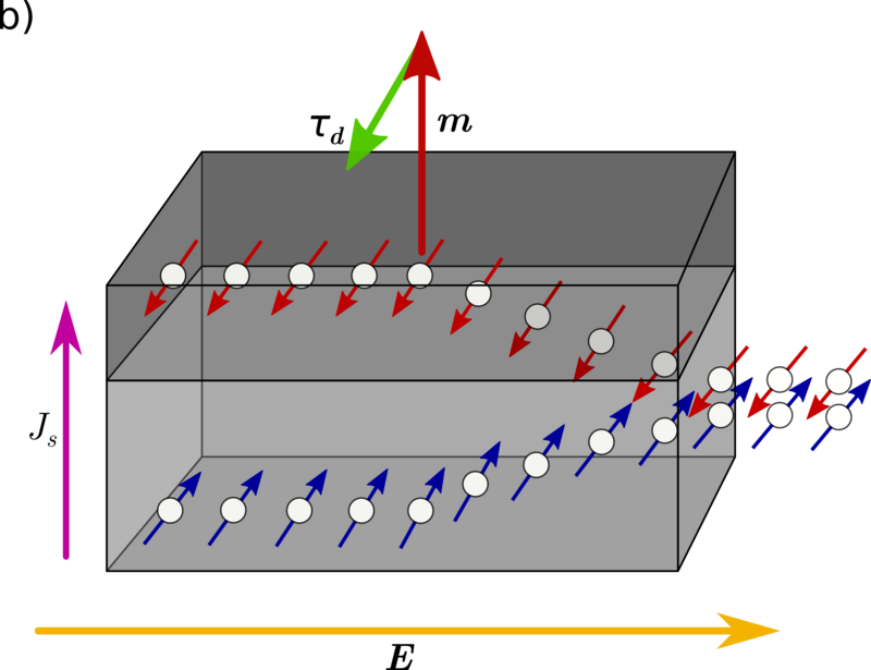
Figure 2.4: Illustration of the SHE in a CIP NM/FM bilayer. An electric field (yellow arrow) drives a charge current in a NM layer with a strong bulk SOC. The SHE deflects electrons with opposite spins (red and blue arrows) in opposite directions, resulting in a transverse spin current (purple arrow). The spin current is injected into the adjacent FM layer, where it exerts a DL torque (green arrow) on the magnetization (red arrow).

Figure 2.4 illustrates the SHE in a NM/FM bilayer. When an in-plane charge current is applied across the NM layer, the SHE filters the electrons based on their spin orientation, resulting in a transverse pure spin current. This spin current is injected into the FM, where it exerts a torque, damping the magnetization towards the direction of spin polarization. The effectiveness of the SHE to convert a charge current into a spin current is typically characterized by the dimensionless spin Hall angle, defined as the ratio of the spin current density to the charge current density in the NM layer.

2.4.2 The Rashba-Edelstein Effect

(image)

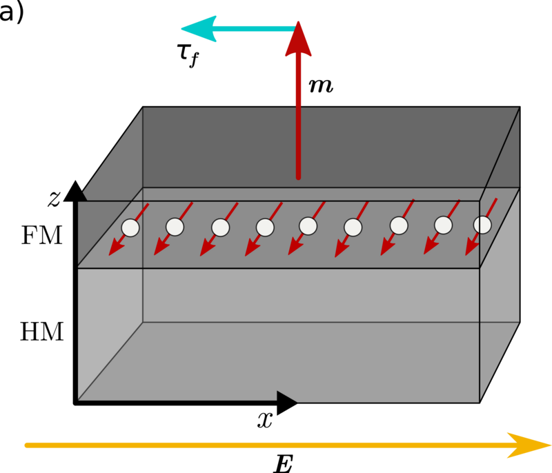
Figure 2.5: Illustration of the REE in a CIP NM/FM bilayer. An in-plane electric field (yellow arrow) is applied across a bilayer system with a Rashba SOC at the interface, resulting in a spin accumulation at the interface through the REE. The spin polarization (red arrows) is perpendicular to both the electric field and the interface normal and results in a FL torque (cyan arrow) on the magnetization (red arrow).

In crystal systems that lack inversion symmetry, the spin degeneracy in the electronic energy bands is lifted by the SOC. In 1955, Dresselhaus studied SOC in the bulk of zinc blende crystals and found that the resulting coupling is an odd function of the electron momentum [41]. A few years later, in 1959, Rashba and Sheka used symmetry-based arguments to derive a similar form of SOC for wurtzite semiconductors [42]. These two types of SOC are now known as the Dresselhaus and Rashba SOCs, respectively. In 1984, Bychkov and Rashba described the spin splitting in two-dimensional (2D) electron gases using the Rashba SOC, successfully explaining the observed electron spin resonance in 2D semiconductors [43]. In 1990, Edelstein proposed a mechanism for generating a non-equilibrium spin accumulation in 2D electron gases with SOC under an applied in-plane electric field [44]. When the SOC takes the Rashba form, this mechanism is referred to as the REE. In 2008, Manchon and Zhang suggested that the REE at FM interfaces could generate torques acting on the magnetization [45]. Later, in 2011, Miron et al. attributed this effect to play a significant role in switching the perpendicular magnetization of a thin Co film in a Pt/Co bilayer capped with AlO\(_x\) [39]. The REE was experimentally demonstrated in 2013 by Rojas Sanchez et al. for a Bi/Ag interface [46].

The SHE could account for the strong DL torques observed in NM/FM bilayers; however, a strong FL torque was also observed, which could not be explained by the SHE alone and showed signs of originating from the NM/FM interface [16]. The REE torques proposed by Manchon and Zhang could account for the strong FL torques; thus, the two mechanisms are often considered to be acting simultaneously in NM/FM bilayers. The REE in a NM/FM bilayer and the resulting SOT are illustrated in Fig. 2.5. When an in-plane electric field is applied across the bilayer, the Rashba SOC at the NM/FM interface generates a spin accumulation through the REE. The resulting spin polarization direction is perpendicular to both the electric field and the interface normal, just like for the SHE. This spin accumulation interacts with the magnetization of the adjacent FM layer, exerting a FL torque on it.

(image)

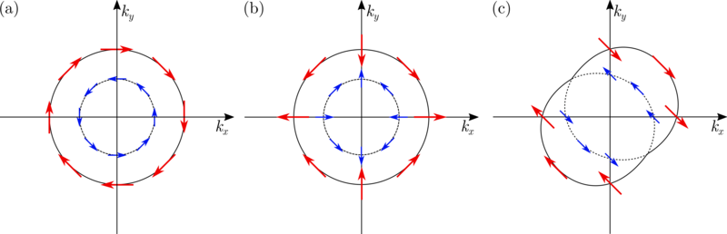
Figure 2.6: The Fermi-level spin texture for different SOCs. (a) Rashba SOC, (b) Linear Dresselhaus SOC, and (c) the combination of both SOCs with equal magnitude.

The Dresselhaus and Rashba SOCs are the two most widely studied forms of SOC in systems with broken inversion symmetry. The polarization direction of the spin accumulation generated by these SOCs can be understood by considering their Hamiltonians. The linear Dresselhaus Hamiltonian is given by

\begin{equation} \hat {H}_D = \beta _D(\sigma _x k_x - \sigma _y k_y), \end{equation}

while the Rashba Hamiltonian is given by

\begin{equation} H_R = \alpha _R\boldsymbol {\sigma }\cdot (\boldsymbol {k}\times \boldsymbol {z}/z), \end{equation}

where \(\beta _D\) and \(\alpha _R\) are the strengths of the interactions [47]. The resulting Dresselhaus and Rashba spin-orbit fields point along \((kx,-ky,0)\) and \(\boldsymbol {k}\times \boldsymbol {z}\), respectively. The Fermi-level spin textures resulting from these two spin-orbit fields are shown in Fig. 2.6 together with a linear combination of both. When an electric field is applied, the carrier occupations are biased in the direction of the field, resulting in a net spin polarization.