The total magnetic Gibbs free energy of a FM system \(\epsilon \) contains several contributions depending on the material and its properties. Some contributions are quantum mechanical in origin, while others are described by
classical magnetostatics. Stable magnetization configurations are reached when all the contributions to the Gibbs energy are in equilibrium, and are found by minimizing the total energy of the system while constraining the
magnetization to the unit sphere:
where \(\delta \epsilon /\delta \bm {m}\) is the functional derivative of the Gibbs free energy with respect to the magnetization. Consequently, the minimization of the energy necessitates that the magnetization is aligned
with the effective field; thus, the LLG describes a process where the system relaxes to a state with minimal energy. In the following subsections, the contributions to the effective field considered in this work, and their respective
energies, are presented.
3.2.1 External Field
The external field \(\bm {H_\mathrm {ext}}\) describes the contribution from all fields applied to the system from outside it. The corresponding energy contribution, often referred to as Zeeman energy, reads [54]
where the integral is over the volume of the magnetic domain \(\omega \).
3.2.2 Exchange Field
In FM materials, the localized magnetic moments are coupled to each other through the quantum mechanical exchange interaction. For two spins, the exchange interaction energetically prefers a parallel alignment, as described by
the Heisenberg Hamiltonian:
where \(J_{ij}\) is the exchange coupling constant between two unit spins \(\bm {S_i}\) and \(\bm {S_j}\) at lattice sites \(i\) and \(j\). By considering the continuous magnetization field \(\bm {m}(\bm {r})\) at site \(\bm
{r}\), and its exchange energy with all other sites in the system, it can be shown that the exchange energy is given by [54]
where \(A_\mathrm {exch} \) is referred to as the exchange stiffness, a material-dependent constant capturing the strength of the exchange interaction. Using equation (3.11), yields
where \(\Delta \) is the Laplace operator. The exchange field acts to align the magnetization uniformly, penalizing inhomogeneous configurations of the magnetization distribution.
3.2.3 The Dzyaloshinskii-Moriya Interaction (DMI)
In certain material systems, Dzyaloshinskii and Moriya discovered that neighbouring spins can interact through the SOC, causing an antisymmetric exchange interaction referred to as the Dzyaloshinskii-Moriya interaction (DMI).
In contrast to the Heisenberg exchange interaction, the DMI prefers an orthogonal alignment of the spins, as described by its Hamiltonian:
where the coupling vector \(\bm {D_{ij}}\) depends on the symmetry of the system.
In magnetic materials which lack inversion symmetry in their bulk, the coupling vector is given by \(\bm {d_{ij}} = -D\bm {\hat {r}_{ij}}\), where \(D\) is a coupling constant, and \(\bm {\hat {r}_{ij}}\) is the unit
vector pointing from spin site \(i\) to spin site \(j\). This form of antisymmetric exchange is referred to as the bulk DMI. It can be shown that the energy contribution from the bulk DMI is given by [54]
together with the BC \(\partial _{\bm {n}} \bm {m} = -D_\mathrm {bdmi}/(2A_\mathrm {exch})\bm {m} \times \bm {n} \), where \(\bm {n}\) is the interface normal of the boundary. The strength of the bulk DMI is
captured by the material parameter \(D_\mathrm {bdmi}\).
Another form of the DMI appears when a FM layer is in contact with a material with a strong SOC, such as a HM. In this case, the DMI is referred to as interface DMI, and the coupling vector is given by \(\bm {D_{ij}} =
-D(\bm {\hat {r}_{ij}}\times \bm {n_d})\), where \(\bm {n_d}\) is the normal of the interface with the HM. The energy contribution from the interface DMI is given by [54]
and the corresponding BC reads \(\partial _{\bm {n}} \bm {m} = -D_\mathrm {idmi}(2A_\mathrm {exch})\left (\bm {n_d}\times \bm {n}\right ) \times \bm {m} \).
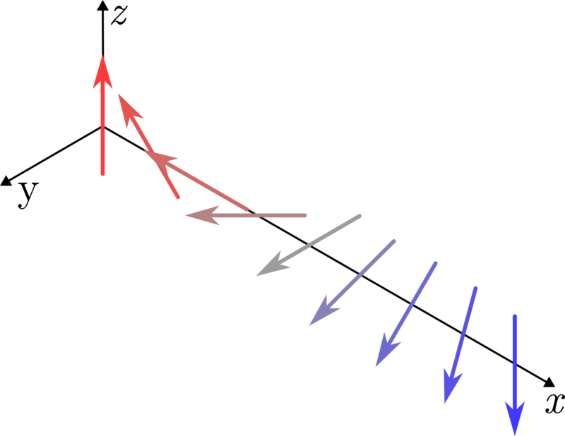
(a) Bloch domain wall.
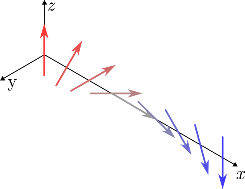
(b) Néel domain wall.
Figure 3.2: A sketch of Bloch and Néel type domain walls. The Bloch wall (a) has a magnetization that rotates in the plane of the wall, while the Néel wall (b) has a magnetization that rotates out of the plane of the wall.
The combination of the DMI and the exchange interactions leads to the spins favoring a canted orientation with respect to each other, which is crucial for the formation of stable chiral magnetic configurations such as skyrmions and
domain walls. These structures can be either of the Bloch or Néel type, depending on whether the DMI is of bulk or interface form, respectively. These two types of domain walls are sketched in Fig. 3.2.
3.2.4 Anisotropy Field
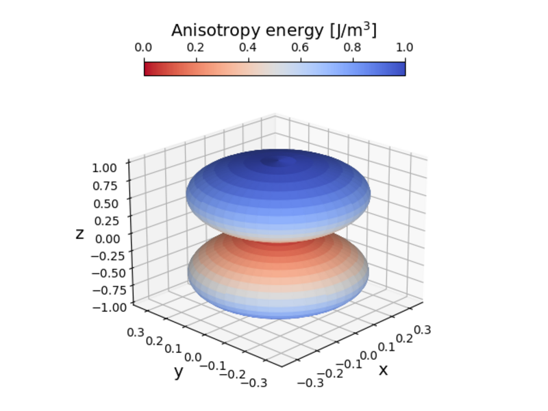
(a) Planar uniaxial anisotropy.
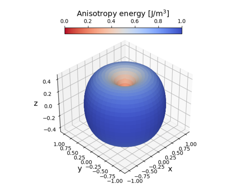
(b) Perpendicular uniaxial anisotropy.
Figure 3.3: The uniaxial anisotropy energy of a single spin projected onto the unit sphere. The easy axis is along the \(z\)-axis, the anisotropy constants are \(K_1 = K_2 = -0.5 \,\unit {J/m^3}\) for (a), and \(K_1 = K_2
= 0.5 \,\unit {J/m^3}\) for (b), resulting in a planar and perpendicular anisotropy, respectively. To obtain a total energy with a positive sign in (b), an isotropic energy contribution \(\epsilon _\mathrm {iso} = 1 \,\unit
{J/m^3}\) is added to the uniaxial anisotropy energy.
In certain materials and systems, the magnetization prefers to align along or away from one or more so-called easy axes. This property is referred to as magnetic anisotropy and is attributed to the SOC from anisotropies in the
crystal structure or at materials interfaces. When the system has a single easy axis \(\bm {e_A}\), the anisotropy energy is given by [54]
where \(K_1\) and \(K_2\) are the first and second order anisotropy constants, respectively. When \(K_{1/2} > 0\), it is energetically favorable for the magnetization to align along the easy axis, while when \(K_{1/2} <
0\), the magnetization prefers to align perpendicular to the easy axis. Neglecting the higher order contributions, the effective field contribution from the uniaxial anisotropy energy is given by
The energy contribution from the dipole-dipole interactions in a magnetic system energetically favors a state with a minimal magnetic moment. The contribution can be expressed as
where \(\bm {H_d}\) is a field acting to reduce the total magnetic moment of the material, often referred to as the demagnetizing field. As the demagnetizing field is generated by the magnetization itself, it depends on the
geometry of the magnetic system and the magnetization distribution.
The magnetostatic Maxwell equations read
\(\seteqnumber{1}{3.24}{0}\)
\begin{align}
\bm {H} & = \frac {1}{\mu _0}\bm {B} - \bm {M},\label {eq:def_of_H} \\ \nabla \cdot \bm {B} & = 0,\label {eq:div_of_B} \\ \nabla \times \bm {H} & = \bm {J_e}.
\end{align}
The demagnetizing field \(\bm {H_d}\) is independent of the electrical current; therefore, it satisfies
\(\seteqnumber{1}{3.25}{0}\)
\begin{align}
\nabla \cdot \bm {H_{d}} & = -\nabla \cdot \bm {M},\label {eq:div_Hd} \\ \nabla \times \bm {H_{d}} & = 0, \label {eq:curl_of_Hd}
\end{align}
where the divergence of Eq. (3.24a) was used together with Eq. (3.24b).
Equation (3.25b) implies that the demagnetizing field is conservative and can be described as the gradient of a scalar potential \(u\), i.e. \(\bm
{H_{d}} = -\nabla u\). The scalar potential is determined by Eq. (3.25a) together with the conditions for the open boundary and the boundary of the
magnetic domain. Therefore, it satisfies the following system of equations:
\(\seteqnumber{1}{3.26}{0}\)
\begin{align}
-\nabla ^2u & = -M_S\bm {\nabla }\cdot \bm {m} & & \text {inside } \omega , \\ -\nabla ^2u & = 0 & & \text {outside } \omega , \\ \left [u\right ] & = 0 & &
\text {at } \partial \omega , \\ \left [\nabla u\right ] & = -\bm {M}\cdot \bm {n} & & \text {at } \partial \omega , \\ u(\bm {r}) & = \mathcal {O}\left (1/r^{2} \right ) &
& \text {outside } \omega \text { as } r\rightarrow \infty ,
\end{align}
where \(\partial \omega \) denotes the boundary of the magnetic domain, and \([u] = u_\mathrm {inside}-u_\mathrm {outside}\) is the jump of the potential across the boundary of the domain. A general solution of this
system of equations reads [54]
where \(\rho (\bm {r'}) = -M_S\bm {\nabla }\cdot \bm {m}(\bm {r'})\), and \(\sigma (\bm {r'}) = M_s\bm {m}(\bm {r'})\cdot \bm {n}\). The demagnetizing field can then be computed from
Computing the demagnetizing field can be challenging due to the long-range interactions between magnetic moments, and its presence outside magnetic domains. Thus, most numerical approaches focus on computing the scalar
magnetic potential \(u\) by solving its Poisson equation (3.26), and then taking its gradient, instead of computing the field directly with
Eq. (3.28) [55].