

Modeling Spin-Orbit Torques
in Advanced Magnetoresistive Devices
6.5 Weak Formulation of the LLG Equation
A FM domain \(\omega \) with boundary \(\partial \omega \) is considered. Including both the bulk and interface DMI fields, the problem can be formulated as follows:
\(\seteqnumber{1}{6.70}{0}\)\begin{align} \partial _t \bm {m} & = -\gamma _0\bm {m}\times \bm {H_\mathrm {eff}}(\bm {m}) + \alpha \bm {m}\times \partial _t \bm {m} + \frac {1}{M_s}\bm {T_s}(\bm {m}) & & \text {in } \omega , \\ \partial _{\bm {n}} \bm {m} & = -\frac {D_{\mathrm {idmi}}}{2A_{\mathrm {exch}}} (\bm {n_d}\times \bm {n}) \times \bm {m} -\frac {D_{\mathrm {bdmi}}}{2A_{\mathrm {exch}}} \bm {m}\times \bm {n} & & \text {on } \partial \omega , \\ \bm {m}(0) & = \bm {m^0} & & \text {in } \omega , \end{align} where \(\bm {m^0} \) is the initial condition for the magnetization at \(t = 0\).
To simulate the time evolution of the magnetization, it is often convenient to solve the LLG equation for the time derivative of the magnetization in order to calculate the magnetization at the next time step. To simplify the notation: \(\bm {v} \coloneqq \partial _t \bm {m}\). Since the magnetization is normalized \(\vert \vert \bm {m} \vert \vert = 1\), the magnetization varies only in the plane perpendicular to \(\bm {m}\), thus \(\bm {m}\cdot \bm {v} = 0\). Solutions \(\bm {v}\) are therefore sought in the vector space
\(\seteqnumber{0}{6.}{70}\)\begin{equation} V_T = \{ \bm {w}\in \bm {H^1}(\omega ):\bm {m}\cdot \bm {w} = 0 \}, \end{equation}
on the domain \(\omega \). Again, the notation \(\bm {w}\in \bm {H^1}(\omega )\) denotes that each component of the vector \(\bm {w}\) belongs to \(H^1(\omega )\).
Taking the cross product of the LLG equation with the magnetization yields
\(\seteqnumber{0}{6.}{71}\)\begin{equation} \bm {m}\times \bm {v} = -\gamma _0\bm {m}\times \left [\bm {m}\times \bm {H_\mathrm {eff}(\bm {m})}\right ] + \alpha \bm {m}\times \left (\bm {m}\times \bm {v}\right ) + \frac {1}{M_s}\bm {m}\times \bm {T_s}(\bm {m}). \end{equation}
Using the vector triple cross product identity \(\bm {a}\times \left (\bm {b}\times \bm {c}\right ) = \left (\bm {c}\cdot \bm {a}\right )\bm {b} - \left (\bm {a}\cdot \bm {b}\right )\bm {c}\) and collecting the terms containing \(\bm {v}\) on the left-hand side gives
\(\seteqnumber{0}{6.}{72}\)\begin{equation} \label {eq:llg_fem_problem} \alpha \bm {v} + \bm {m}\times \bm {v} = \gamma _0\bm {H_\mathrm {eff}}(\bm {m}) - \gamma _0\left [\bm {H_\mathrm {eff}}(\bm {m})\cdot \bm {m}\right ]\bm {m} + \frac {1}{M_s}\bm {m}\times \bm {T_s}(\bm {m}). \end{equation}
Finally, multiplying Eq. (6.73) with the test function \(\bm {w} \in V\) and integrating over the domain gives the weak formulation of the LLG equation: Find \(\bm {v} \in V_T\) such that
\(\seteqnumber{0}{6.}{73}\)\begin{equation} \label {eq:llg_weak_form_1} \langle \alpha \bm {v} + \bm {m}\times \bm {v}, \bm {w}\rangle _\omega = \gamma _0\langle \bm {H_\mathrm {eff}}(\bm {m}),\bm {w} \rangle _\omega + \frac {1}{M_s}\langle \bm {m}\times \bm {T_s}(\bm {m}),\bm {w} \rangle \qquad \,\forall \, \bm {w} \in V, \end{equation}
where the compact notation \(\langle \bm {f},\bm {g} \rangle _\omega = \int _{\omega } \bm {f}\cdot \bm {g} d\bm {r}\) is used again.
6.5.1 Exchange Term and DMI Boundary Conditions
The effective field term contains several contributions; most thereof can be inserted directly into Eq. (6.74), except for the exchange field due to the second-order derivative. The exchange field contribution reads
\(\seteqnumber{0}{6.}{74}\)\begin{equation} \langle \bm {H_\mathrm {exch}}(\bm {m}),\bm {w} \rangle _\omega = \frac {2A_\mathrm {exch}}{\mu _0 M_s}\langle \Delta \bm {m},\bm {w} \rangle _\omega = \frac {2A_\mathrm {exch}}{\mu _0 M_s} \left (\langle \partial _{\bm {n}}\bm {m},\bm {w}\rangle _{\partial \omega } - \langle \nabla \bm {m},\nabla \bm {w} \rangle _\omega \right ), \end{equation}
where integration by parts was applied. The normal derivative of the magnetization in the boundary term can now be replaced with the BCs for the interfacial and bulk DMI fields:
\(\seteqnumber{0}{6.}{75}\)\begin{equation} \langle \bm {H_\mathrm {exch}}(\bm {m}),\bm {w} \rangle _\omega = -\frac {2A_\mathrm {exch}}{\mu _0 M_s}\langle \nabla \bm {m},\nabla \bm {w} \rangle _\omega . -\frac {D_{\mathrm {bdmi}}}{\mu _0 M_s} \langle \bm {m}\times \bm {n},\bm {w}\rangle _{\partial \omega } -\frac {D_{\mathrm {idmi}}}{\mu _0 M_s} \langle (\bm {n_d}\times \bm {n}) \times \bm {m},\bm {w}\rangle _{\partial \omega } \end{equation}
From integration by parts, it can be shown that \(\langle \bm {a}\times \bm {n},\bm {b}\rangle _{\partial \Omega } = \langle \bm {a},\nabla \times \bm {b}\rangle _\Omega - \langle \nabla \times \bm {a},\bm {b}\rangle _\Omega \). By using this identity, the boundary terms can be converted into volume terms:
\(\seteqnumber{0}{6.}{76}\)\begin{equation} \label {eq:exchange_field_weak_form} \langle \bm {H_\mathrm {exch}}(\bm {m}),\bm {w} \rangle _\omega = -\frac {2A_\mathrm {exch}}{\mu _0 M_s}\langle \nabla \bm {m},\nabla \bm {w} \rangle _\omega + \frac {D_{\mathrm {idmi}}}{\mu _0 M_s} \langle (\nabla \times \bm {n_d}) \times \bm {m},\bm {w}\rangle _{\omega } +\frac {D_{\mathrm {bdmi}}}{\mu _0 M_s} \langle \nabla \times \bm {m},\bm {w}\rangle _{\omega } -\frac {D_{\mathrm {idmi}}}{\mu _0 M_s} \langle \bm {m}, (\nabla \times \bm {n_d}) \times \bm {w}\rangle _{\omega } -\frac {D_{\mathrm {bdmi}}}{\mu _0 M_s} \langle \bm {m},\nabla \times \bm {w}\rangle _{\omega }. \end{equation}
The second and third term can be written \(-\frac {1}{2}\langle \bm {H_\mathrm {idmi}}(\bm {m}),\bm {w} \rangle _\omega - \frac {1}{2}\langle \bm {H_\mathrm {bdmi}}(\bm {m}),\bm {w} \rangle _\omega \), while the fourth and fifth can be written \(\frac {1}{2}\langle \bm {m},\bm {H_\mathrm {idmi}}(\bm {w}) \rangle _\omega + \frac {1}{2}\langle \bm {m},\bm {H_\mathrm {bdmi}}(\bm {w})\rangle _\omega \). Inserting Eq. (6.77) into the effective field term in Eq. (6.74) gives the weak formulation: find \(\bm {v} \in V_T\) such that
\(\seteqnumber{0}{6.}{77}\)\begin{multline} \label {eq:llg_weak_form_2} \alpha \langle \bm {v}, \bm {w}\rangle _\omega + \langle \bm {m}\times \bm {v}, \bm {w}\rangle _\omega = \frac {\gamma _0}{2}\langle \bm {H_\mathrm {idmi}}(\bm {m}),\bm {w} \rangle _\omega + \frac {\gamma _0}{2}\langle \bm {m},\bm {H_\mathrm {idmi}}(\bm {w}) \rangle _\omega + \frac {\gamma _0}{2}\langle \bm {H_\mathrm {bdmi}}(\bm {m}),\bm {w} \rangle _\omega + \frac {\gamma _0}{2}\langle \bm {m},\bm {H_\mathrm {bdmi}}(\bm {w}) \rangle _\omega -\gamma _0\frac {2A_\mathrm {exch}}{\mu _0 M_s}\langle \nabla \bm {m},\nabla \bm {w} \rangle _\omega \\ +\gamma _0\langle \bm {H_\mathrm {ext}}+\bm {H_\mathrm {aniso}}(\bm {m})+\bm {H_\mathrm {demag}}(\bm {m}),\bm {w} \rangle _\omega + \frac {1}{M_s}\langle \bm {m}\times \bm {T_s}(\bm {m}),\bm {w} \rangle \forall \, \bm {w} \in V_T. \end{multline} After having solved for \(\bm {v}\), the magnetization at the next time step can be estimated depending on the time integration scheme used.
6.5.2 Bulk and Interface Spin Torque
If the spin torque is computed using the charge and spin drift-diffusion equations, the torque in the FM layers at time step \(i\) is given by
\(\seteqnumber{0}{6.}{78}\)\begin{equation} \bm {T_s}(\bm {m^i}) = -D_e\left [\frac {\bm {m^i}\times \bm {S^i}}{\lambda _J^2} + \frac {\bm {m^i}\times \left (\bm {m^i}\times \bm {S^i}\right )}{\lambda _\phi ^2}\right ], \end{equation}
where \(\bm {S^i}\) is the spin accumulation at time step \(i\) computed with \(\bm {m^i}\). The contribution to the linear form of the LLG equation is given by
\(\seteqnumber{0}{6.}{79}\)\begin{equation} \frac {1}{M_s}\langle \bm {m^i}\times \bm {T_s}(\bm {m^i}),\bm {w} \rangle = -\frac {D_e}{M_s \lambda ^2_J}\langle \bm {S^i} ,\bm {w}\rangle _\omega -\frac {D_e}{M_s \lambda ^2_\phi } \langle \bm {m^i}\times \bm {S^i},\bm {w}\rangle _\omega , \end{equation}
where the vector triple cross product identity was used together with \(\bm {m^i}\cdot \bm {w} = 0\).
If the interface magnetism BCs are considered, the torque acting on the magnetization at the interface must be included. For an NM/FM interface at \(z=0\) the interfacial torque is given at time step \(i\) by
\(\seteqnumber{0}{6.}{80}\)\begin{equation} \bm {T^\mathrm {int}_s}(\bm {m^i}) = \tilde {\Gamma }^\mathrm {mag}(\bm {m^i})\left (\bm {V_s^{F,i}} + \bm {V^{N,i}_s}\right )\delta (z) + \bm {\gamma ^\mathrm {mag}}(\bm {m^i})\delta (z). \end{equation}
The delta function can be omitted by including the interfacial torque as a boundary term in the weak formulation of the LLG equation. The interfacial torque contribution to the linear form of the LLG equation is thus given by
\(\seteqnumber{0}{6.}{81}\)\begin{equation} \frac {1}{M_s}\langle \bm {m^i}\times \bm {T^\mathrm {int}_s}(\bm {m^i}),\bm {w} \rangle _\omega = \frac {1}{M_s}\langle \bm {m^i}\times \left [\tilde {\Gamma }^\mathrm {mag}(\bm {m^i})\left ( \bm {V_s^{F,i}} + \bm {V_s^{N,i}}\right )\right ],\bm {w}\rangle _{\Gamma _\mathrm {eff|F}} + \frac {1}{M_s}\langle \bm {m^i}\times \bm {\gamma ^\mathrm {mag}}(\bm {m^i}),\bm {w}\rangle _{\Gamma _\mathrm {eff|F}}, \end{equation}
where \(\Gamma _\mathrm {eff|F}\) is the interface shared by the FM and the effective interface layer.
6.5.3 First Order Tangent-Plane Scheme
In order to compute the time evolution of the magnetization over a given time period \(T\), the time is discretized such that \(t_i = ih\) for \(0 \leq i \leq N\), and \(T = Nh\), where \(h\) is the time step. At any time-step \(t_{i}\) the FEM approximation of Eq. (6.78) is solved for \(\bm {v}\) using the approximate magnetization solution \(\bm {m^{i} } \approx \bm {m}(t_{i} )\). The magnetization at the next time step \(t_{i+1} \) is then given by
\(\seteqnumber{0}{6.}{82}\)\begin{equation} \bm {m^{i+1}} = \frac {\bm {m^i} + h \, \bm {v}}{\left |\left |\bm {m^i} + h \, \bm {v}\right |\right |}, \end{equation}
where the division by the norm ensures that the magnetization remains normalized. This time integration scheme is referred to as the explicit tangent-plane scheme [89].
The tangent-plane scheme can be made implicit by replacing the magnetization in the weak formulation with
\(\seteqnumber{0}{6.}{83}\)\begin{equation} \bm {m} = \bm {m^{i}} + \theta h \bm {v}, \end{equation}
where \(\theta \) is the degree of implicitness, with \(0 \leq \theta \leq 1\). For \(\theta = 0\) the scheme is explicit, while for \(\theta = 1\) it is fully implicit. Typically, this substitution is only made for the exchange field term, resulting in one additional term in the bilinear form. The tangent-plane scheme with implicit exchange term thus gives the final weak formulation of the LLG equation considered in this work: find \(\bm {v}\in V_T\) such that
\(\seteqnumber{0}{6.}{84}\)\begin{multline} \alpha \langle \bm {v}, \bm {w}\rangle _\omega + \langle \bm {m^i}\times \bm {v}, \bm {w}\rangle _\omega + \theta h\gamma _0\frac {2A_\mathrm {exch}}{\mu _0 M_s}\langle \nabla \bm {v},\nabla \bm {w} \rangle _\omega = \frac {\gamma _0}{2}\langle \bm {H_\mathrm {idmi}}(\bm {m^i}),\bm {w} \rangle _\omega + \frac {\gamma _0}{2}\langle \bm {m^i},\bm {H_\mathrm {idmi}}(\bm {w}) \rangle _\omega \\ + \frac {\gamma _0}{2}\langle \bm {H_\mathrm {bdmi}}(\bm {m^i}),\bm {w} \rangle _\omega + \frac {\gamma _0}{2}\langle \bm {m^i},\bm {H_\mathrm {bdmi}}(\bm {w}) \rangle _\omega -\gamma _0\frac {2A_\mathrm {exch}}{\mu _0 M_s}\langle \nabla \bm {m^i},\nabla \bm {w} \rangle _\omega +\gamma _0\langle \bm {H_\mathrm {ext}}+\bm {H_\mathrm {aniso}}(\bm {m^i})+\bm {H_\mathrm {demag}}(\bm {m^i}),\bm {w} \rangle _\omega + \frac {1}{M_s}\langle \bm {m^i}\times \bm {T_s}(\bm {m^i}),\bm {w} \rangle \\ \forall \, \bm {w} \in V_T. \end{multline}
6.5.4 Implementation of the LLG Equation
The LLG equation is implemented in the in-house simulation software ViennaSpinMag [86]. The LLG module of the software has been extended through this work to include both the bulk and interface DMI fields, as well as the interface torques. The resulting linear system of equations from the weak formulation of the LLG is due to the cross products, again solved using the GMRES method provided by the MFEM library. The demagnetization field contribution is calculated on the magnetic domains using a hybrid method combining the FEM with the boundary element method (BEM) [90, 91], for more details on the implementation see [55].
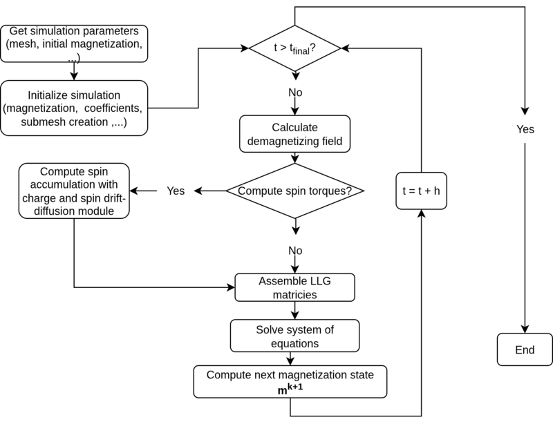
Figure 6.13 shows the flow chart of the LLG module in ViennaSpinMag. The software takes in a mesh of the system, which can contain both NM and FM regions. The LLG module creates a new mesh (submesh) containing only the FM regions of the original mesh on which the demagnetization field and the LLG equation are computed. If the spin torques are included, the charge and spin drift-diffusion equations are solved first on the full mesh to obtain the spin accumulation. The spin accumulation is then used to compute the spin torque acting on the magnetization. The time evolution of the magnetization is computed using the tangent-plane scheme with a fully implicit exchange term \(\theta =1\). The simulation proceeds until the time \(t_\mathrm {final}\) is reached, or until a stopping criterion is met, e.g., the magnetization has converged to a stable state.
In the next two subsections, the accuracy and the validity of the DMI implementation in the LLG equation are assessed through two numerical tests.
6.5.5 One-Dimensional Problem
To validate the implementation of the LLG equation with DMI, the numerical test from Ref. [92] is reproduced. In this test, a simple 1D problem is considered. For a 1D magnetic system limited to the region \(x\in [-L/2,L/2]\). Minimizing the energy of the system using the variational calculus yields the following ordinary differential equation (ODE) [93, 92]:
\(\seteqnumber{1}{6.86}{0}\)\begin{align} \partial _x^2 \theta & = \frac {\sin (\theta )\cos (\theta )}{\Delta ^2} & \text { for } -\frac {L}{2} < x < \frac {L}{2} , \\ \sin (\theta ) & = {\mathbin {\textpm }} \frac {\Delta }{\xi } & \text { for } x = -\frac {L}{2} \text { or } x = \frac {L}{2} ,\label {eq:1dODEb} \end{align} where \(\Delta = \sqrt {A/K_1}\), \(\xi = 2A/D\), and \(\theta \) is the polar angle describing the magnetization direction: \(\bm {m} = (\sin (\theta )\cos (\phi ),\sin (\theta )\sin (\phi ),\cos (\theta ))\). If the DMI is of the interfacial type: \(\phi = 0\), and the sign in Eq. (6.86b) is positive. For the case of bulk DMI: \(\phi = \pi /2\), and the sign is in Eq. (6.86b) negative.
| Parameter | 1D System | FeGe | Unit |
| \(\alpha \) | \(1.0\) | \(0.28\) | \(1\) |
| \(M_s\) | \(0.86\) | \(0.384\) | \(\mathrm {MAm^{-1}}\) |
| \(A\) | \(13.0\) | \(8.78\) | \(\mathrm {pJm^{-1}}\) |
| \(D\) | \(3.0\) | \(1.58\) | \(\mathrm {mJm^{-2}}\) |
| \(K_1\) | \(0.4\) | \(0.0\) | \(\mathrm {mJm^{-2}}\) |
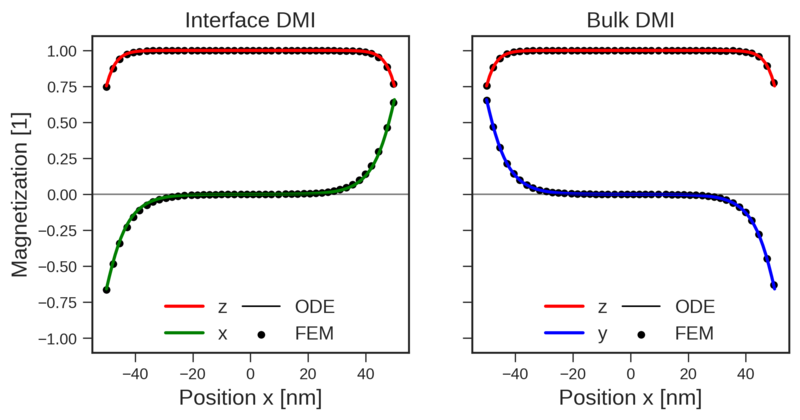
The system size is set to \(L = 50\,\mathrm {nm}\) and the magnetic parameters used for the 1D-system are shown in table 6.2. For both the interfacial and bulk DMI cases, the ODE is solved using the shooting method [83]. Using the FEM implementation of the LLG equation, the system is relaxed to obtain the minimal energy state. The initial magnetization configuration is uniform along the direction \(\bm {m} = \hat {z}\), and the damping parameter \(\alpha = 1.0\) is chosen in order to accelerate the relaxation process. The time step is set to \(h = 0.1\,\mathrm {ps}\), and a quasi 1D mesh is used, with the dimensions \(100 \times 1\times 1 \, \mathrm {nm^3}\) consisting of tetrahedron elements. Figure 6.14 shows the comparison of the ODE and FEM solutions for the interfacial and bulk DMI cases. The FEM solution shows good agreement with the ODE solution, with an AMRE of \(6.38\%\) for the interfacial DMI case and \(0.9\%\) for the bulk DMI case. The error is caused by the Neumann BCs explicitly imposed through the FEM implementation, which introduce effects along the widths of the quasi 1D system that are not included in the ODE. Nonetheless, the results show that the DMI is properly implemented.
6.5.6 Three-Dimensional Problem
To further test the implementation, the numerical experiment from Ref. [94] is reproduced. A \(9\,\mathrm {nm}\) thick helimagnetic nanodisk is considered with an initial state where the magnetization is uniformly oriented along \(\hat {z}\). The diameter is varied between \(80-200\,\mathrm {nm}\), and the material parameters of FeGe are used, shown in table 6.2. The time step is set to \(h = 0.1\,\mathrm {ps}\), and the LLG equation is solved until the magnetization relaxes to a stable state. Again, the damping parameter is set to \(\alpha = 1.0\) to speed up the relaxation process.
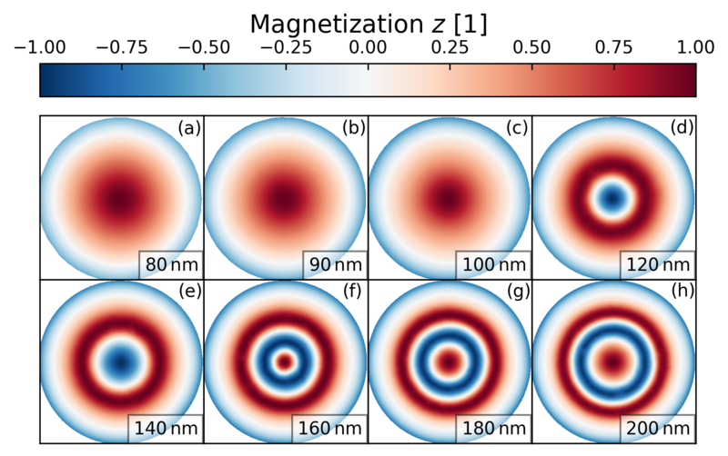
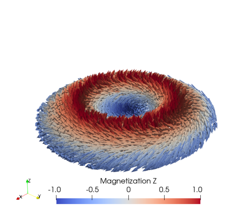
Figure 6.15 shows the relaxed state of the nanodisk for the different diameters. The equilibrium states are radially symmetric isolated skyrmion states for all diameters. For the diameters \(80-100\,\mathrm {nm}\) the skyrmions are incomplete as \(m_z\) does not cover the entire range \([-1,1]\), while for the diameters \(120-140\,\mathrm {nm}\) the skyrmions are complete. For the diameters \(160-200\,\mathrm {nm}\), \(m_z\) covers the interval \([-1,1]\) twice, forming target shaped skyrmions. These results are in exact agreement with the results presented in Ref. [94].
To study the time evolution of the magnetization from an initial state to a relaxed state, it is often convenient to compute the volume-averaged magnetization:
\(\seteqnumber{0}{6.}{86}\)\begin{equation} \bm {\overline {m}} = \frac {1}{V_\omega }\int _\omega \bm {m} d\bm {r}. \end{equation}
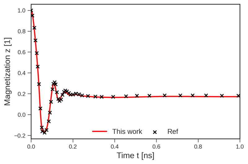
Figure 6.16 shows the time evolution of the volume-averaged \(z\)-component of the magnetization and the final relaxed state of the \(140\,\mathrm {nm}\) nanodisk. The results were obtained using the reported FeGe Gilbert damping parameter \(\alpha = 0.28\), and a uniform magnetization along \(\hat {z}\) as an initial state. The data points were sampled from Ref. [94], where a different time integration scheme was employed. Nonetheless, the time evolution shows an excellent agreement with the results presented in Ref. [94].