

Modeling Spin-Orbit Torques
in Advanced Magnetoresistive Devices
6.3 The Finite Element Method (FEM)
The finite element method (FEM) is a numerical approach for solving PDEs. It is widely used in engineering and mathematical modeling to solve problems in structural analysis, heat transfer, and many other fields. The method involves transforming the problem into a variational problem, discretizing the problem domain into smaller subdomains, and approximating the solution in each subdomain, resulting in a linear system of equations over all the subdomains [85]. The FEM is particularly useful for solving PDEs in systems with complex geometries and with various BCs. Thus, it is well-suited for solving the full 3D charge and spin drift-diffusion equations, as well as the LLG equation. In this section, the FEM and its main concepts are briefly summarized. Furthermore, the treatment of different BCs is presented.
6.3.1 The Weak Formulation
The first step for solving a PDE using the FEM is to derive its weak formulation. As an example, the following Poisson problem for the domain \(\Omega \) is considered:
\(\seteqnumber{0}{6.}{23}\)\begin{equation} -\kappa \nabla ^2 u =f \qquad \text {in } \Omega , \end{equation}
where \(\kappa \) is a constant material parameter and \(u\) is a scalar field potential defined on the domain. At the boundary \(\partial \Omega \), the following BCs are considered on different segments of the boundary:
\(\seteqnumber{1}{6.25}{0}\)\begin{align} u & = u_D \qquad & \text {on } \partial \Omega _D \subset \partial \Omega , \\ \kappa \nabla u \cdot \bm {n} & = u_N \qquad & \text {on } \partial \Omega _N \subset \partial \Omega , \\ \kappa \nabla u \cdot \bm {n} + \alpha u & = u_R \qquad & \text {on } \partial \Omega _R \subset \partial \Omega , \end{align} where \(\bm {n}\) is the outward-pointing normal vector on the boundary, and \(\alpha \), \(u_D\), \(u_N\), and \(u_R\) are different constants. The first condition is a Dirichlet BC, which prescribes the value of \(u\) on the boundary \(\partial \Omega _D\). The second condition is a Neumann BC, which prescribes the normal derivative of \(u\) on the boundary \(\partial \Omega _N\). The third condition is a Robin BC, which combines both Dirichlet and Neumann conditions on the boundary \(\partial \Omega _R\). A 2D sketch of the system is depicted in Fig. 6.5a.

The weak formulation of the problem is obtained by multiplying the equation by a test function \(v \in V\), where \(V\) is a vector space, and integrating over the domain \(\Omega \):
\(\seteqnumber{0}{6.}{25}\)\begin{equation} -\kappa \int _\Omega \nabla ^2 u v\, d\bm {r} = \int _\Omega fv \, d\bm {r}. \end{equation}
By applying the product rule of differentiation and the divergence theorem (integration by parts), the second-order partial derivatives can be transformed into first-order derivatives and a boundary term:
\(\seteqnumber{0}{6.}{26}\)\begin{equation} \label {eq:fem_gauss} \kappa \int _\Omega \nabla u \cdot \nabla v\, d\bm {r} - \kappa \int _{\partial \Omega } \nabla u \cdot \bm {n} v\, d\bm {s} = \int _\Omega fv \, d\bm {r}, \end{equation}
where \(\bm {r}\) and \(\bm {s}\) are the position vectors in the volume and on the surface, respectively. The boundary integral can be split into each segment containing the Dirichlet, Neumann, and Robin BCs. For the unspecified segments of the boundary, so-called natural BCs are implicitly assumed, which do not contribute to the weak formulation, in this case \(\nabla u \cdot \bm {n} = 0\). Inserting these BCs into Eq. (6.27) and collecting the terms independent of \(u\) on the right-hand side yields
\(\seteqnumber{0}{6.}{27}\)\begin{equation} \kappa \int _\Omega \nabla u \cdot \nabla v\, d\bm {r} - \alpha \int _{\partial \Omega _R} u v\, d\bm {s} = \int _\Omega fv \, d\bm {r} - \int _{\partial \Omega _N} u_N v\, d\bm {s} -\int _{\partial \Omega _R} u_R v\, d\bm {s}. \end{equation}
The following functions are defined:
\(\seteqnumber{0}{6.}{28}\)\begin{equation} a(u,v) = \kappa \int _\Omega \nabla u \cdot \nabla v\, d\bm {r} - \alpha \int _{\partial \Omega _R} u v\, d\bm {s}, \end{equation}
and
\(\seteqnumber{0}{6.}{29}\)\begin{equation} l(v) = \int _\Omega fv \, d\bm {r} - \int _{\partial \Omega _N} u_N v\, d\bm {s} -\int _{\partial \Omega _R} u_R v\, d\bm {s}, \end{equation}
which are referred to as the bilinear form and the linear form, respectively. The weak formulation of the problem then reads as follows: find \(u \in V\) such that
\(\seteqnumber{0}{6.}{30}\)\begin{equation} a(u,v) = l(v) \qquad \,\forall \, v \in V. \end{equation}
While the original problem required the solution to be twice differentiable, the weak formulation only requires the solution to be once differentiable, hence the name. The Dirichlet conditions can be directly incorporated into the definition of the vector space that is used to find the solution. The solution then belongs to the space
\(\seteqnumber{0}{6.}{31}\)\begin{equation} V_D = \{ v\in V: v(\bm {r}) = u_D \,\forall \, \bm {r} \in \partial \Omega _D \}. \end{equation}
6.3.2 The Finite Element Approximation
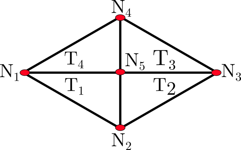
To approximate the solution the domain \(\Omega \) is decomposed into subdomains \(T_i\) called elements, forming a mesh of the domain \(\mathcal {T} \coloneqq \{T_i, i= 1,\dots ,N_T\}\), where \(N_T\) is the number of elements. The endpoints of the elements are called nodes and form the collection \(\mathcal {N} =\{\bm {r_i}: i =1,\dots N_N \}\), where \(N_N\) is the number of nodes. A sketch of a 2D mesh is shown in Fig. 6.5b. On the mesh, a finite dimensional space \(V_h \subset V\) is introduced, which is spanned by the basis functions \(\phi _i\) with the property
\(\seteqnumber{0}{6.}{32}\)\begin{equation} \phi _i(\bm {r_j}) = \delta _{ij} \qquad \,\forall \, \bm {r_j} \in \mathcal {N}, \end{equation}
which are non-zero on the elements adjacent to the node \(\bm {r_i}\) and zero everywhere else. The basis functions depend on the geometry of the elements and the finite element space used; typically, they consist of piecewise polynomials.
The finite element approximation is then defined as follows: find \(u_h \in V_h\) satisfying
\(\seteqnumber{0}{6.}{33}\)\begin{equation} \label {eq:weak_form_fem} a(u_h,v_h) = l(v_h) \qquad \,\forall \, v_h \in V_h. \end{equation}
The solution \(u_h\) can be expressed in terms of the basis functions as
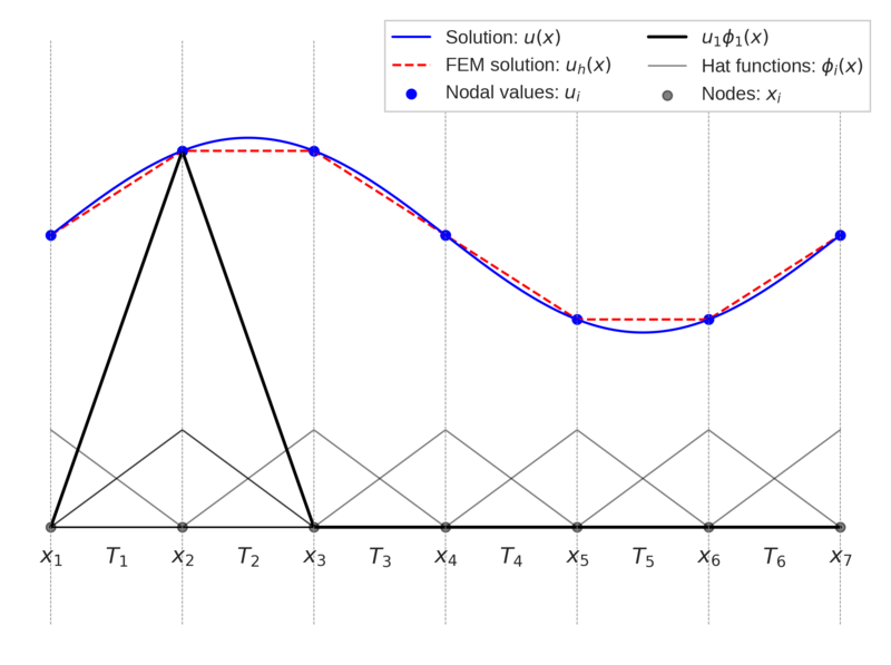
\(\seteqnumber{0}{6.}{34}\)\begin{equation} \label {eq:solution_function} u_h(\bm {r}) = \sum _i u_i \phi _i(\bm {r}), \end{equation}
where \(u_i\) are unknown coefficients to be determined. Figure 6.6 illustrates the approximate solution \(u_h\) for a 1D system with linear basis functions often referred to as hat functions, where the coefficients \(u_i\) are the values of the solution at the nodes.
Inserting Eq. (6.35) into Eq. (6.34) and using the test function \(v_h=\phi _j\) yields
\(\seteqnumber{0}{6.}{35}\)\begin{equation} a\left (\sum _{i} u_i \phi _i,\phi _j\right ) = \sum _{i}u_i a(\phi _i,\phi _j) = l(\phi _j). \end{equation}
Next a matrix \(A\) and vector \(\bm {l}\), referred to as the stiffness matrix and load vector, respectively, are defined:
\(\seteqnumber{0}{6.}{36}\)\begin{equation} A_{ij} \coloneqq a(\phi _j,\phi _i) = \kappa \int _\Omega \nabla \phi _j \cdot \nabla \phi _i \, d\bm {r} -\int _{\partial \Omega _R} \alpha \phi _j \phi _i \, d\bm {s}, \end{equation}
\(\seteqnumber{0}{6.}{37}\)\begin{equation} l_j \coloneqq l(\phi _j) = \int _\Omega f \phi _j \, d\bm {r} - \int _{\partial \Omega _N} u_N \phi _j \, d\bm {s} - \int _{\partial \Omega _R} u_R \phi _j \, d\bm {s}. \end{equation}
The weak formulation can then be written as a linear system of equations:
\(\seteqnumber{0}{6.}{38}\)\begin{equation} A\bm {u} = \bm {l}. \end{equation}
The vector of unknown coefficients is obtained by multiplying the load vector by the inverted stiffness matrix: \(\bm {u} = A^{-1}\bm {l}\). As the stiffness matrix is typically sparse, it can be inverted most efficiently by using iterative methods, thereby avoiding more computationally expensive direct methods such as LU factorization.
To account for the Dirichlet BCs, the system can be expressed
\(\seteqnumber{0}{6.}{39}\)\begin{equation} \begin{pmatrix} I & 0 \\ A_{FD} & A_{FF} \end {pmatrix} \begin{pmatrix} \bm {u}_D \\ \bm {u}_F \end {pmatrix} = \begin{pmatrix} \bm {u}_D \\ \bm {l}_F \end {pmatrix}, \end{equation}
where \((A_{FD})_{ij}\) is the bilinear form where \(\phi _j\) belongs to the nodes at the Dirichlet boundary with known coefficients \((\bm {u_D})_j\), while \(\phi _i\) belongs to the "free" nodes where the coefficients \((\bm {u_F})_i\) are unknown. The matrix \((A_{FF})_{ij}\) is the bilinear form where both \(\phi _i\) and \(\phi _j\) belong to the free nodes, and \((\bm {l}_F)_i\) is the corresponding load vector. The solution is then given by
\(\seteqnumber{0}{6.}{40}\)\begin{equation} \bm {u}_F = -A_{FF}^{-1}A_{FD}\bm {u}_D + A_{FF}^{-1}\bm {l}_F. \end{equation}
6.3.3 Internal Boundaries
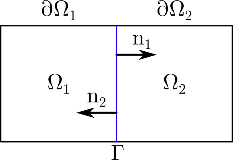
If the domain \(\Omega \) can be split into two subdomains \(\Omega _1\) and \(\Omega _2\) with different material parameters \(\kappa _1\) and \(\kappa _2\), respectively, the weak formulation presented above still holds for each domain. The total bilinear and linear forms are then obtained by summing the bilinear and linear forms of each subdomain. However, as the internal boundary \(\Gamma \) between the two subdomains is part of the outer boundary of each subdomain, two additional boundary terms for this interface are obtained in the weak formulation:
\(\seteqnumber{0}{6.}{41}\)\begin{equation} \label {eq:fem_internal_boundary} a_\Gamma = \kappa _2\int _{\Gamma } \nabla u_2 \cdot \bm {n_2} v_2\, d\bm {s} +\kappa _1\int _{\Gamma } \nabla u_1 \cdot \bm {n_1} v_1\, d\bm {s}, \end{equation}
where \(\bm {n_i}\), \(u_i\), and \(v_i\) are the normal vectors, potentials, and test functions at the internal boundary belonging to \(\Omega _i\) for \(i =1,2\), respectively. The system is depicted in Fig. 6.7. Since \(\bm {n_2} = - \bm {n_1}\) one can write
\(\seteqnumber{0}{6.}{42}\)\begin{equation} \label {eq:fem_internal_boundary_2} a_\Gamma = \int _{\Gamma } \bm {J_2}\cdot \bm {n_1} v_2\, d\bm {s}-\int _{\Gamma } \bm {J_1}\cdot \bm {n_1} v_1\, d\bm {s}, \end{equation}
where the currents \(\bm {J}_i = -\kappa _i\nabla u_i\) for \(i = 1,2\) are introduced. The currents can be expressed in terms of averages and differences: \(\bm {J_1} = \bm {\overline {J}} - \Delta \bm {J}/2 \) and \(\bm {J_2} = \bm {\overline {J}} + \Delta \bm {J}/2\), where \(\bm {\overline {J}} = (\bm {J_2} + \bm {J_1})/2\) is the average current and \(\Delta \bm {J} = \bm {J_2} - \bm {J_1}\) is the difference between the currents across the interface. This gives
\(\seteqnumber{0}{6.}{43}\)\begin{equation} \label {eq:fem_internal_boundary_3} a_\Gamma =-\frac {1}{2}\int _{\Gamma } (2\bm {\overline {J}} - \Delta \bm {J} )\cdot \bm {n_1} v_1\, d\bm {s} + \frac {1}{2}\int _{\Gamma } (2\bm {\overline {J}} + \Delta \bm {J} )\cdot \bm {n_1} v_2\, d\bm {s} = \int _{\Gamma } \bm {\overline {J}} \cdot \bm {n_1} \Delta v\, d\bm {s} + \int _{\Gamma } \Delta \bm {J} \cdot \bm {n_1} \overline {v}\, d\bm {s}, \end{equation}
where \(\Delta v = v_2 - v_1\) and \(\overline {v} = (v_2 + v_1)/2\) are the difference and average of the test functions on the internal boundary, respectively.
If the potentials and currents are required to be continuous across the internal boundary, i.e., \(u_1 = u_2\) and \(j_1 = j_2\), both of the interface terms vanish. If the potentials or currents are not continuous across the internal boundary, a finite element space that allows for discontinuities at the internal interfaces is required. Furthermore, the FEM discretization requires an additional set of nodes on the internal boundary, as each side of the interface must have its own set of nodes. FEMs with additional interface nodes are referred to as extended or enriched FEMs.
6.3.4 Effective Interface Layer Approximation
A simple method for capturing solutions with discontinuities at the internal boundaries is to model the interface with an effective interface layer. By introducing a thin effective interface layer \(\Omega _{eff}\) of thickness \(d_{eff}\) between the two domains, where the solution is approximated by a linear function, the discontinuities in the solution can then be captured by typical continuous finite element spaces without requiring additional extended FEMs.
By treating the interface as an effective layer, the average testfunction across the interface \(\overline {v} = (v_1+v_2)/2\) in Eq. (6.44) can then be approximated by the mean of the testfunction over the thickness of the effective interface layer:
\(\seteqnumber{0}{6.}{44}\)\begin{equation} \label {eq:average_test_function} \overline {v} \approx \frac {1}{d_{eff}}\int _{-\frac {d_{eff} }{2}}^{\frac {d_{eff} }{2}} v\, dl. \end{equation}
The difference across the interface is given by the fundamental theorem of calculus for line integrals:
\(\seteqnumber{0}{6.}{45}\)\begin{equation} \label {eq:delta_test_function} \Delta v = \int _{-\frac {d_{eff} }{2}}^{\frac {d_{eff} }{2}} \bm {n_1}\cdot (\nabla v)\, dl. \end{equation}
Inserting Eqs. (6.45) and (6.46) into the internal boundary term (6.44) gives
\(\seteqnumber{0}{6.}{46}\)\begin{equation} a_{\Omega _{eff}} = \int _{\Omega _{eff} } \bm {\overline {J}} \cdot \bm {n_1} \left [\bm {n_1}\cdot (\nabla v)\right ]\, d\bm {r} + \frac {1}{d_{eff} }\int _{\Omega _{eff} } \Delta \bm {J} \cdot \bm {n_1} v, \,d\bm {r}, \end{equation}
where \(\int _\Gamma \int _{-d_{eff} /2}^{d_{eff} /2} d\bm {s}dl = \int _{\Omega _{eff}} d\bm {r} \) was used.
In some cases, the currents defined on the internal boundaries depend on the average and difference of the potentials across the interface, as in the BCs for the drift-diffusion equations presented in the previous chapter. Considering \(\bm {\overline {J}} = a\Delta u\) and \(\Delta \bm {J} = b\overline {u}\), where \(a\) and \(b\) are interface dependent scalar parameters. Inside the effective interface layer, the average and difference of the potentials are approximated with \(\overline {u} \approx u\) and \(\Delta u \approx d_{eff}[\bm {n_1}\cdot (\nabla u)]\), respectively. The internal BCs then read
\(\seteqnumber{0}{6.}{47}\)\begin{equation} a_{\Omega _{eff}} = d_{eff} a\int _{\Omega _{eff} } \left [\bm {n_1}\cdot (\nabla u)\right ]\left [\bm {n_1}\cdot (\nabla v)\right ]\, d\bm {r} + \frac {b}{d_{eff} }\int _{\Omega _{eff} } u v \,d\bm {r}, \end{equation}
and must be included in the final bilinear form.
6.3.5 Connected Interlayer Boundaries
If the two subdomains \(\Omega _1\) and \(\Omega _2\) are separated by a layer where the scalar field does not exist, such as the TB in a MTJ, two additional boundary terms are introduced, one for each interface between the subdomains and the interlayer. The contribution to the weak formulation from these internal boundaries is given by
\(\seteqnumber{0}{6.}{48}\)\begin{equation} \label {eq:fem_connected_internal_boundary} \kappa _2\int _{\Gamma _1} \nabla u_2 \cdot \bm {n_2} v_2\, d\bm {r} +\kappa _1\int _{\Gamma _2} \nabla u_1 \cdot \bm {n_1} v_1\, d\bm {r} = -\int _{\Gamma _1} \bm {J_2}\cdot \bm {n_2} v_2\, d\bm {r}-\int _{\Gamma _2} \bm {J_1}\cdot \bm {n_1} v_1\, d\bm {r}, \end{equation}
where the currents \(\bm {J_1}\) and \(\bm {J_2}\) are defined on the internal boundaries \(\Gamma _1\) and \(\Gamma _2\), respectively.